Task Graph

Contents

1 Problem
2 Context
3 Forces
4 Solution
5 Variations
6 Examples
7 Known Uses
8 Related Patterns
9 Acknowledgements
10 References
11 Appendix — Understanding the C# Examples

Problem

Many computational problems can be considered to be a static collection of atomic tasks with dependencies between their inputs and outputs. On completion, tasks terminate and their output is used as input to other (dependent) tasks. The tasks and their dependencies may be known at compile time or just prior to execution of the tasks. In many cases the tasks may be of variable size resulting in varying execution times. Tasks may have multiple input dependencies and create output that forms the input to many other (dependent) tasks. The tasks can be thought of as forming the vertices of a directed acyclic graph while the graph’s directed edges show the dependencies between tasks.

How do we create a programming model that exposes the underlying parallelism of the collection of tasks and executes efficiently, executing tasks in parallel or serially depending on when inputs become available? The Task Graph pattern addresses this problem.

Note: The Task Graph pattern presented here should not be confused with the Arbitrary Static Task Graph architectural pattern (3), which addresses the overall organization of the program.

Context

Problems that can be broken down into atomic tasks, as described above, can be implemented as graph of tasks with dependencies between them. Each task is a separate unit of work that may take dependencies on one or more antecedents (see Figure 1 below). Tasks with antecedents may only start when all their antecedents have completed. The result of an antecedent task may be passed to dependent tasks on completion of the antecedent. Data does not stream to dependents during execution, the antecedent completes its work, terminates, and then its result is passed to the dependents. The final result of the graph is returned when the last dependent task(s) complete (tasks C, E, and F in bold in Figure 1 below).

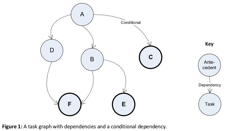
Figure 1 shows task dependencies. Thus, tasks B and D are dependent on task A, their antecedent, and cannot start until task A completes. A task may be dependent on multiple antecedents (in the diagram above F is dependent on B and D). The graph is acyclic—the dependencies between tasks are one way—meaning that tasks cannot impose further dependencies on their antecedents.

Task graphs are defined statically at design time (see the Variations and Examples sections for alternatives). Even though the graph is statically defined, it is possible for tasks to be conditional on the outcome of an antecedent. In Figure 1 task C only executes if some condition of task A is met. So a task graph may exhibit some dynamic behavior at run time depending on whether a condition is met, but all the tasks and dependencies of the graph are known at compile time. Different frameworks and run-times may support different conditions, e.g. on error, on completion/non-completion, on cancellation (4).

This pattern requires a framework that allows the programmer to define tasks, specify dependencies and when to wait on task completion, and a runtime which can execute the graph. In the .NET 4 Framework this is implemented by the Task Parallel Library (TPL) (1). The TPL provides an API containing a factory for creating tasks and specifying their dependencies. Tasks are units of work that may be executed on a single thread. The TPL runtime schedules tasks on a queue and executes them on a pool of threads, blocking tasks until their dependencies are met. See the Examples section for implementations using the TPL and the Known Uses section for other similar implementations.

Forces

Universal forces

Task Graph vs. Other patterns – See the Related Patterns section for a discussion of how Task Graph differs from other (seemingly) similar patterns such as Pipeline and Divide and Conquer. Depending on the scenario other patterns may be simpler to implement and offer other advantages such as automatic load balancing.
Variable vs. Uniform task size – Breaking down the problem into a graph containing tasks of roughly uniform execution time may be harder but will usually result in a more efficient implementation. A graph which contains highly variable task sizes, e.g. many smaller (quick) tasks and one or two very large (long running) tasks will typically result in an overall execution time dominated by the larger tasks and is unlikely to be very efficient. Overall a few very small tasks is probably acceptable, but you don’t want too many of them, you also don’t want your biggest task to be a lot bigger than any of the others.
Large vs. Small tasks – A graph of very small task sizes, even if uniform, may also be inefficient. The task creation and management overhead becomes significant relative to the amount of work carried out by the task. Conversely, if the tasks are too big, there won’t be enough parallelism and lots of time is wasted waiting for the biggest task to finish.
Problem size vs. Graph overhead – The problem must be large enough to justify the overhead of creating the graph. For problems with very small numbers of small tasks, the cost of creating a graph may be too great and result in a very inefficient implementation with little or no speedup over a serial version.
Compile time vs. Run time defined graphs – Compile time defined graphs represent the simplest usage of the pattern but also place significant limitations on its applicability as all tasks and dependencies must be known up front. For problems where the task breakdown is only known at run time, a dynamically defined task graph is required. Task graphs defined at run time may exploit more of the available parallelism of the problem but also add to the complexity of the solution. See the Variations section for further discussion.

Implementation forces

Task breakdown vs. Hardware capacity — Implementations of the Task Graph pattern may create an arbitrary number of tasks. This may be more than the number of processing elements (PEs) available in hardware. Implementations may limit the number of tasks created to avoid oversubscription of PEs, or reuse PEs for subsequent tasks but limit the number of tasks being executed simultaneously. Conversely, creating fewer tasks than the number of available PEs will result in underutilization. Efficient implementations usually create significantly more tasks than PEs as this allows the scheduler to load- balance and allows for some scalability if more PEs become available. This is particularly important for task graphs with non-uniform task sizing.
Task granularity vs. Startup & communication overhead — Depending on the communication cost between processing elements and the startup and execution overheads for a task, using larger grained tasks will reduce communication and task creation overhead. Smaller grained tasks may result in better load balancing but the application will waste time creating and communicating with them.
Task granularity vs. Startup latency – Depending on the startup cost of creating tasks or assigning them to processing elements, implementations may use larger grained tasks to reduce overhead when starting new tasks. Finer grained tasks may result in better load balancing at the expense of additional startup cost and resource usage. Frameworks reduce startup latency by reusing PEs from a pool at the expense of additional management overhead and possibly maintaining unused PEs.

Solution

The solution to problems of this type is to break down the computation into a series of atomic tasks with clearly defined dependencies to form a directed acyclic graph. The acyclic nature of the graph is important as it removes the possibility of deadlocks between tasks, provided the tasks are truly atomic. When specifying the graph it is really important to understand all dependencies between tasks, hidden dependencies may result in deadlocks or races. The runtime schedules tasks according to their dependencies and executes them on the available PEs. The overall task graph is considered complete when all the tasks have completed.

Break down the problem using the Task Decomposition, Group Tasks and Order Tasks patterns to decompose the tasks and analyze the dependencies and non-dependencies between them (see: Patterns for Parallel Programming, Chapter 3 (2)). In summary:

Task Decomposition – Identify atomic tasks that can execute concurrently.

Group Tasks – Group tasks to identify temporal dependencies and truly atomic tasks.

Order Tasks – Identify how tasks must be ordered to satisfy constraints among tasks.

This approach may lead to several different possible graphs. Use the Design Evaluation pattern (see: Patterns for Parallel Programming, Chapter 3 (2)) to assess the appropriateness of each proposed task graph for the target hardware. In summary:

How many PEs are available? A task breakdown that results in many more tasks than PEs usually results in a more efficient implementation. However additional tasks represent additional overhead which may reduce the overall efficiency. Eventually the overhead of managing too many tasks will dominate the computation.

How much data is passed between tasks? Does the proposed task graph use the right level of task granularity based on communication latency and bandwidth.

Is the proposed design flexible, efficient and as simple as possible? These may be conflicting requirements especially if more than one target platform is under consideration.

At run time tasks are then assigned to a pool of PEs based on the task dependencies and the availability of PEs (see the Examples section).

Load Balancing. The resulting task graph does not inherently load balance the computation (like Master/Worker). Tasks may be of differing sizes, which may result in bottlenecks depending on the layout of the graph. The load characteristic of the graph is determined by the critical path through the slowest tasks. The Task Graph pattern does nothing to resolve this issue; this issue is left to the programmer implementing the graph. The programmer can remove bottlenecks by either breaking down the slowest tasks into additional tasks on the graph which can execute in parallel or by modifying the task such that it executes in parallel internally.

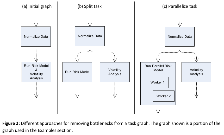
In Figure 2 (a) the Run Risk Model and Volatility Analysis task represents one such bottleneck in a larger graph discussed in the Examples section. The programmer can choose to break out different parts of task; Run Risk Model and Volatility Analysis and add them as separate tasks on the graph (b). They could also choose to parallelize the Run Risk Model internally because it cannot be broken down into atomic tasks or is more amenable to parallelization with another pattern (for example Master/Worker). Both of these approaches may be used together (c).

Sharing Data. There are two approaches to sharing data between tasks when using this pattern. Data can be synchronized explicitly by passing data from antecedents to dependents. It is also possible to take a control flow synchronization approach and simply use the dependencies to control when tasks execute and access shared data.

The data synchronization approach results in a clearer separation of data dependencies but may reduce inefficiency if large amounts of data need to be copied. Using control flow synchronization takes advantage of the shared data at the expense of clarity which may lead to correctness errors.

Error Handling. Individual tasks must handle any errors and the programmer must consider how to deal with errors and propagate error state back to the application if necessary. They may choose to do this in a number of ways. In some cases ignoring errors or returning an alternative result on error might be acceptable. Another approach would be to return error information by adding additional flags or data to the task result or by using features specific to the implementation language or framework. For example, the Task Parallel Library aggregates exceptions from tasks within the graph into an AggregateException exception (4) that is thrown and handled by the code that created the graph.

Variations

In some programs the number of tasks and their dependencies may not be known until run time. This is a common occurrence when using the Task Graph pattern. In this case the programmer can specify the graph at run time. This may be as simple as modifying a graph by adding a few additional tasks to it based on (user) input conditions, or as complex as creating the entire graph. This variation increases the number of problems to which the Task Graph pattern can be applied. It may also result in programs that exploit more of the available concurrency. However, it also adds to the complexity and maintainability of the solution, and places more of a burden on the programmer to ensure correctness.

It is important to realize that even in these cases the task graph does not evolve during execution. Tasks do not create other dependent tasks. Conditional tasks may be present in the graph but the task and the conditions under which it executes are defined by the program prior to execution of the graph.

Figure 3 shows a task graph for a wavefront calculation on a grid of variable size. The calculation for grid element (m, n) is dependent on elements (m-1, n) and (m, n-1) but the overall size of the grid is only known at run time.

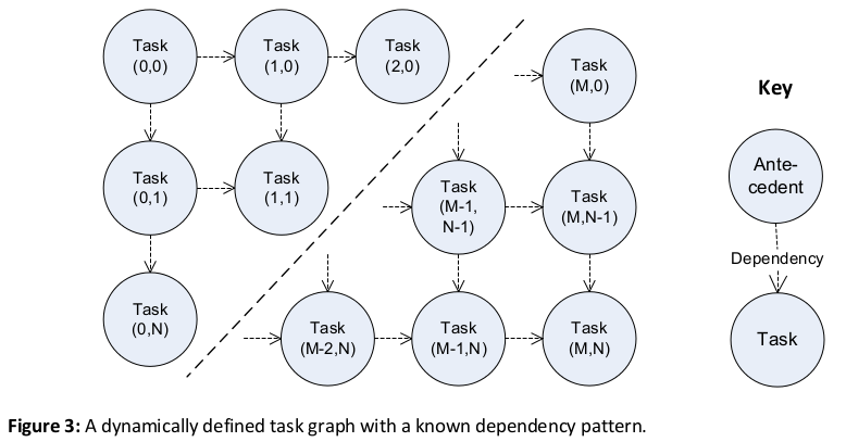
See the Examples section for an implementation of the graph in Figure 3. See the Known Uses section for further discussion of applications which use task graphs that are defined at run time.

Examples

Here is a hypothetical system that loads both current (last trading period) and historical financial data from different sources and runs a risk model against both sets of data before comparing the result to verify the model’s relevance to current trading conditions. This is not a real time trading system waiting for stock updates in real time as discussed by Joshi (5). In this application large datasets are used to assess overall market conditions and the graph is created and executed each time the user asks for an analysis.

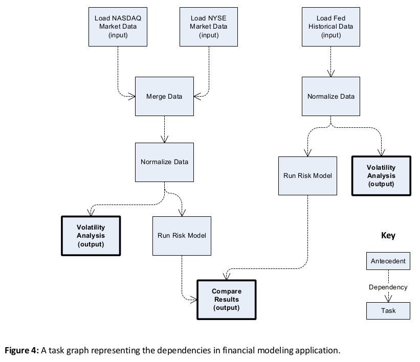
Figure 4 shows task dependencies. Thus, the task “Merge Data” is dependent on tasks “Load NASDAQ Market Data” and “Load NYSE Market Data.” The program reports volatility statistics for market and historical data as well as comparing models. These three results (the bold boxes) may be returned in any order as the graph does not specify any dependencies between the tasks.

This task breakdown can be expressed as a task graph in C# using the .NET Framework 4 Task Parallel Library (TPL) (1) and is targeted at a multi-core processor. For clarity the example code below defines the graph, but the code for the actual tasks is not shown. Readers unfamiliar with C# and the TPL should read Appendix A for a brief discussion of the code.

class Program
{
    // Actual work done by the tasks methods not shown here.
    private static MarketData LoadNyseData() { /* ... */ } 
    private static MarketData LoadNasdaqData() { /* ... */ } 
    private static MarketData LoadFedHistoricalData(){ /* ... */ }
    private static MarketData NormalizeData(Task<MarketData>[] tasks) { /* ... */ } 
    private static MarketData MergeMarketData(Task<MarketData>[] tasks) { /* ... */ } 
    private static AnalysisResult AnalyzeData(Task<MarketData>[] tasks) { /* ... */ } 
    private static ModelResult ModelData(Task<MarketData>[] tasks) { /* ... */ } 
    private static void CompareModels(Task<ModelResult>[] tasks) { /* ... */ }

    static void Main(string[] args)
    {
        TaskFactory factory = Task.Factory;

        Task<MarketData> loadNyseData = Task<MarketData>.Factory.StartNew(
            () => LoadNyseData(), TaskCreationOptions.LongRunning);

        Task<MarketData> loadNasdaqData = Task<MarketData>.Factory.StartNew(
            () => LoadNasdaqData(), TaskCreationOptions.LongRunning);

        Task<MarketData> mergeMarketData = 
            factory.ContinueWhenAll<MarketData, MarketData>(
                new[] { loadNyseData, loadNasdaqData },
                (tasks) => MergeMarketData(from t in tasks select t.Result));

        Task<MarketData> normalizeMarketData = mergeMarketData.ContinueWith(
            (t) => NormalizeData(t.Result));

        Task<MarketData> loadFedHistoricalData =
            Task<MarketData>.Factory.StartNew(
                () => LoadFedHistoricalData(), TaskCreationOptions.LongRunning);

        Task<MarketData> normalizeHistoricalData = 
            loadFedHistoricalData.ContinueWith(
                (t) => NormalizeData(t.Result));

        Task<MarketAnalysis> analyzeMarketData = 
            normalizeMarketData.ContinueWith(
                (t) => AnalyzeData(t.Result));

        Task<MarketModel> modelMarketData = 
            analyzeMarketData.ContinueWith(
                (t) => CreateModel(t.Result));

        Task<MarketAnalysis> analyzeHistoricalData = 
            normalizeHistoricalData.ContinueWith(
                (t) => AnalyzeData(t.Result));

        Task<MarketModel> modelHistoricalData = 
            analyzeHistoricalData.ContinueWith(
                (t) => CreateModel(t.Result));

        Task<MarketRecommendation> compareModels = 
            factory.ContinueWhenAll<MarketModel, MarketRecommendation>(
                new[] { modelMarketData, modelHistoricalData },
                (tasks) => CompareModels(from t in tasks select t.Result));

        Task.WaitAll(analyzeHistoricalData, analyzeMarketData, compareModels);
    }
 }

The TPL distributes the tasks across threads running on the available cores, using task continuations to start new tasks as their antecedents complete. Further discussion of the code in this example can be found in “A Guide to Parallel Programming,” Chapter 5 (6).

How does this example resolve the forces? The graph is defined at compile time and contains tasks of variable size. There are more tasks than PEs available on the target platform, a quad core desktop machine, and the graph contains enough work so that the startup and communication overhead does not dominate. The two model tasks are significantly larger than the other tasks, so they account for most of the computation and constrain the efficiency of the graph. Some moderate speedup will be seen from the parallelization, possibly enough to satisfy the productivity programmer. Further parallelization of the modeling tasks—as discussed under Load Balancing in the Solution section—may be required to fully utilize the available cores.

Variation Example: A Graph Defined at Run Time with Known Dependency Pattern
The second example is of a graph that is defined at run time, similar to the one shown in Figure 2. It applies a method, processRowColumnCell(int a, int b), to each element in an integer matrix of size numRows by numColumns. The method accesses only the values of the cells above and to the left, and calculates a new value for cell [a, b] based on them.

public static void GridUpdate(int numRows, int numColumns,
        Action<int, int> processRowColumnCell)
    {
        Task[] prevTaskRow = new Task[numColumns]; 
        Task prevTaskInCurrentRow = null;

        for (int row = 0; row < numRows; row++)
        {
            prevTaskInCurrentRow = null;
            for (int column = 0; column < numColumns; column++)
            {
                int j = row, i = column;

                Task curTask;
            if (row == 0 && column == 0)
            {
                curTask = Task.Factory.StartNew(() => processRowColumnCell(j, i));
            }
            else if (row == 0 || column == 0)
            {
                var antecedent = (column == 0) ? prevTaskRow[0] : prevTaskInCurrentRow; 
                curTask = antecedent.ContinueWith(p =>
                {
                    processRowColumnCell(j, i);
                });
            }
            else
            {
                var antecedents = new Task[] { prevTaskInCurrentRow, prevTaskRow[column] };
                curTask = Task.Factory.ContinueWhenAll(antecedents, ps =>
                {
                    processRowColumnCell(j, i);
                });
            }

            // Keep track of the task just created for future iterations
            prevTaskRow[column] = prevTaskInCurrentRow = curTask;
        }
    }

    // Wait for the last task to be done.
    prevTaskInCurrentRow.Wait();
}

For clarity error handling code has been left out of both these samples. For further examples of task graphs and other the patterns supported by the Task Parallel Library see Toub 2009 (7).

How are the forces resolved? The task graph is defined at run time and depends on the size of the user specified grid dimensions. Assuming the grid is of any realistic size there will be many more tasks than PEs. The tasks are all of uniform size, provided the work being done by processRowColumnCell in each task is sufficiently large, the overhead of creating and managing the graph will be insignificant. The resulting graph will be efficient with good speedup and scaling characteristics over a serial implementation. The graph uses control flow synchronization and passes elements of a shared array to processRowColumnCell . This reduces the amount of data being passed between tasks but introduces the possibility of changes to the code introducing correctness errors.

Known Uses

The Task Graph pattern is used in a number of instances.

For example, build tools create dynamically defined task graphs based on component dependencies and then build components based on ordering. They create graphs where neither the graph’s size nor dependency pattern is known at run time. MSBuild (8) is one such system. MSBuild defines a build process as a group of targets each with clearly defined input and outputs using an XML file. The MSBuild execution engine then generates a task graph and executes it. The executables compiled by one target forming the inputs to subsequent dependent target.

The following frameworks and associated runtimes support the implementation of this pattern:

The .NET 4 Task Parallel Library implements this pattern using Continuation Tasks (4)
The StarSs programming model (9).
Intel® Threading Building Blocks (10).
Dryad also supports the Task Graph pattern although it adds additional support for streaming data between tasks (11).

Related Patterns

Arbitrary Static Task Graph (structural pattern) – Addresses the overall organization of the program rather than an implementation on specific programming model(s).

Task Decomposition, Order Tasks & Group Tasks – The task decomposition, order tasks, and group tasks patterns detail an approach to understanding task dependencies. They help the implementer to specify the directed graph prior to implementation (2).

Several other common patterns bear similarities to Task Graph but actually differ in important respects:

Pipeline – Differs in several important respects from a task graph. Firstly, all pipelines have a fixed (linear) shape with some slight variation for non-linear pipelines. Secondly, the pattern focuses on data flow, rather than task dependencies. Data flows through a pipeline with the same task being executed on multiple data items. Finally, pipelines are usually synchronous with data moving from task to task in lockstep.

Master/Worker – Tasks within the Master/Worker pattern have a child/parent rather than antecedent/dependent relationship. The master task creates all tasks, passes data to them, and waits for a result to be returned. Worker tasks typically all execute the same computation against different data. The number of workers may vary dynamically according to the problem size and number of available PEs.

Divide and Conquer – Tasks within the divide and conquer pattern have a child/parent rather than antecedent/dependent relationship. The resulting task tree is dynamic with the application creating only the root task. All sub-tasks are created by their parent during computation based on the state of the parent. Data is passed from parent to child tasks; the parent then waits for children to complete and may receive results from its children. So, data can move bi-directionally between parent and children, rather than being passed one way from antecedent to dependent.

Discrete Event – Focuses on raising events or sending messages between tasks. There is no limitation on the number of events a task raises or when it raises them. Events may also pass between tasks in either direction; there is no antecedent/dependency relationship. The discrete event pattern could be used to implement a task graph by placing additional restrictions upon it.

Acknowledgements

The author would like to thank the following people for their specific feedback on this paper; Tasneem Brutch (Samsung Electronics, US R&D Center), Ralph Johnson (UIUC), Kurt Keutzer (UC Berkeley) and Stephen Toub and Rick Molloy (Microsoft Corporation) and the attendees of ParaPLoP 2010 who workshopped the paper and RoAnn Corbisier (Microsoft Corporation) for editing the final document.

References

1. Microsoft Corporation. Task Parallel Library. MSDN. [Online] [Cited: March 1, 2010.] http://msdn.microsoft.com/en-us/library/dd460717(VS.100).aspx.

2. Tim Mattson, Beverly A. Sanders and Berna L. Massingill. Patterns for Parallel Programming. s.l. : Addison- Wesley, 2004. ISBN 978-0321228116 .

3. Kurt Keutzer, Tim Mattson. Our Pattern Language (OPL). A Pattern Language for Parallel Programming ver2.0. [Online] 10 14, 2009. [Cited: May 1, 2010.] http://parlab.eecs.berkeley.edu/wiki/_media/patterns/opl- new_with_appendix-20091014.pdf.

4. Microsoft Corporation. Continuation Tasks. MSDN. [Online] [Cited: March 1, 2010.] http://msdn.microsoft.com/en-us/library/ee372288(VS.100).aspx.

5. Concurrent Evaluation of a Directed Acyclic Graph. Joshi, Rakesh. Carefree : s.n., 2010.

6. Microsoft patterns & practices group. A Guide to Parallel Programming: Design Patterns for Decomposition, Coordination and Scalable Sharing. CodePlex. [Online] [Cited: April 1, 2010.] http://parallelpatterns.codeplex.com/.

7. Toub, Stephen. Patterns for Parallel Programming: Understanding and Applying Parallel Patterns with the
.NET Framework 4. Microsoft Download Center. [Online] [Cited: March 1, 2010.] http://www.microsoft.com/downloads/details.aspx?FamilyID=86b3d32b-ad26-4bb8-a3ae-c1637026c3ee.

8. Microsoft Corporation. MSBuild Task. MSDN. [Online] [Cited: March 4, 2010.] http://msdn.microsoft.com/en- us/library/z7f65y0d.aspx.

9. Barcelone Supercomputing Center. SMP superscalar. Barcelone Supercomputing Center. [Online] [Cited: March 4, 2010.] http://www.bsc.es/plantillaG.php?cat_id=385.

10. Intel Corporation. Intel® TBB. Intel® Software Network. [Online] [Cited: April 1, 2010.] http://software.intel.com/en-us/intel-tbb/.

11. Microsoft Corporation. Dryad. Microsoft Research. [Online] [Cited: March 1, 2010.] http://research.microsoft.com/en-us/projects/dryad/.

12. —. The C# Language. Visual C# Developer Center. [Online] [Cited: May 1, 2010.] http://msdn.microsoft.com/en-us/vcsharp/aa336809.aspx.

Appendix — Understanding the C# Examples

The examples in the paper are written using the C# language (12) and the Task Parallel Library (1). To help the reader who is unfamiliar with these technologies a brief walkthrough of key parts of the first example is given here. This appendix is intended to be a brief overview. Further discussion of C#, the TPL, and this example can be found in “A Guide to Parallel Programming”, Chapter 5 (6).

The TPL creates a new factory which supports the creation and scheduling of Task objects. In the TPL a Task is a unit of work that will be scheduled by the runtime to execute on a single thread within a thread pool maintained by the runtime.

TaskFactory factory = Task.Factory;

The example uses the Factory.StartNew method to create a new task that returns a MarketData type. The method is passed an Action containing the work to be done. Here the work is defined as an anonymous delegate, () => LoadNyseData() which calls the LoadNyseData method. In this example the method also passed TaskCreationOptions.LongRunning to provide additional information to the Scheduler that the task may run for a significant period of time.

    Task<MarketData>.Factory.StartNew( (
        ) => LoadNyseData(), 
        TaskCreationOptions.LongRunning);

New tasks can be defined that take dependencies on other tasks. In the code shown below, a new mergeMarketData task is created that takes dependencies on the loadNyseData and loadNasdaqData tasks. The merge task is again defined using an anonymous delegate which is passed an array of antecedent tasks.

    Task<MarketData> mergeMarketData = 
        factory.ContinueWhenAll<MarketData, MarketData>(
            new[] { loadNyseData, loadNasdaqData },
            (tasks) => MergeMarketData(from t in tasks select t.Result));

Tasks can also be defined in terms of their antecedents. Here a new task, modelMarketData, is defined as a dependent of the task analyzeMarketData. Again an anonymous delegate is used to specify the work carried out by the new task; (t) => CreateModel(t.Result). The delegate is passed the antecedent task, t, and the anonymous delegate passes the result of the task, t.Result to the CreateModel method.

    Task<MarketModel> modelMarketData = 
        analyzeMarketData.ContinueWith(
            (t) => CreateModel(t.Result));

Finally the program calls the WaitAll method to ensure that all tasks have completed before it continues.

Task.WaitAll(analyzeHistoricalData, analyzeMarketData, 
    compareModels);