
Statistical Relational Learning
Pedro Domingos
Dept. of Computer Science & Eng. University of Washington
« Statistical Relational Learning
Pedro Domingos
Most machine learning algorithms assume that data points are i.i.d. (independent and identically distributed), but in reality objects have varying distributions and interact with each other in complex ways. Domains where this is prominently the case include the Web, social networks, information extraction, perception, medical diagnosis/epidemiology, molecular and systems biology, ubiquitous computing, and others. Statistical relational learning (SRL) addresses these problems by modeling relations among objects and allowing multiple types of objects in the same model. This tutorial will cover foundations, key ideas, state-of-the-art algorithms and applications of SRL.
Scroll with j/k | | | Size
1
Overview
Motivation Foundational areas
Probabilistic inference Statistical learning Logical inference Inductive logic programming
Putting the pieces together Applications
2
Motivation
Most learners assume i.i.d. data (independent and identically distributed)
One type of object Objects have no relation to each other
Real applications: dependent, variously distributed data
Multiple types of objects Relations between objects
3
Examples
Web search Information extraction Natural language processing Perception Medical diagnosis Computational biology Social networks Ubiquitous computing Etc.
4
Costs and Benefits of SRL
Benefits
Better predictive accuracy Better understanding of domains Growth path for machine learning Learning is much harder Inference becomes a crucial issue Greater complexity for user
Costs
5
Goal and Progress
Goal: Learn from non-i.i.d. data as easily as from i.i.d. data Progress to date
Burgeoning research area Were close enough to goal Easy-to-use open-source software available
Lots of research questions (old and new)
6
Plan
We have the elements:
Probability for handling uncertainty Logic for representing types, relations, and complex dependencies between them Learning and inference algorithms for each
Figure out how to put them together Tremendous leverage on a wide range of applications
7
Disclaimers
Not a complete survey of statistical relational learning Or of foundational areas Focus is practical, not theoretical Assumes basic background in logic, probability and statistics, etc. Please ask questions Tutorial and examples available at alchemy.cs.washington.edu
8
Overview
Motivation Foundational areas
Probabilistic inference Statistical learning Logical inference Inductive logic programming
Putting the pieces together Applications
9
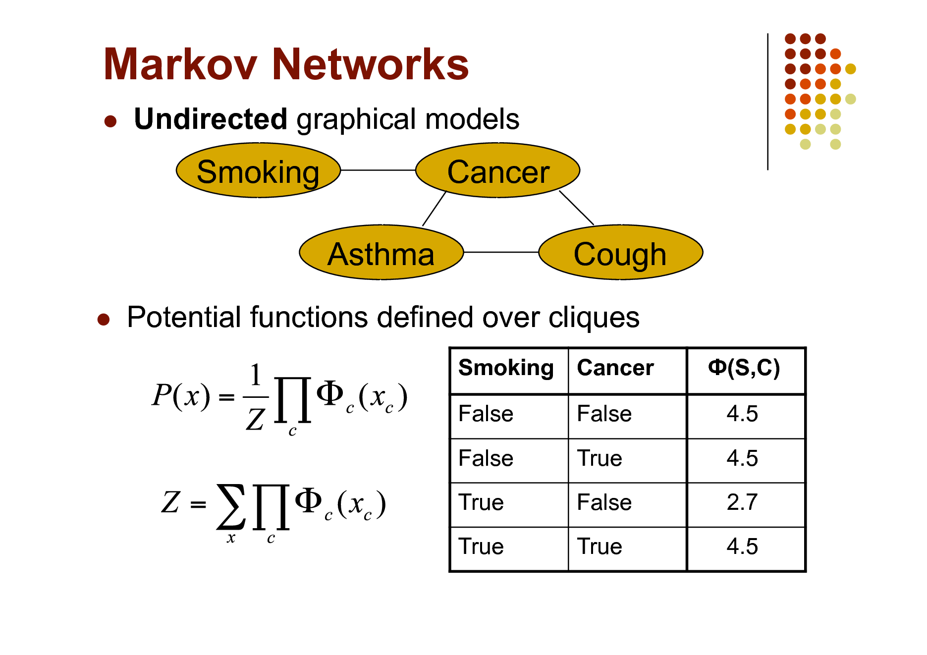
Markov Networks
Undirected graphical models
Smoking Asthma
Cancer Cough
Potential functions defined over cliques
Smoking Cancer False False True True False True False True (S,C) 4.5 4.5 2.7 4.5
10
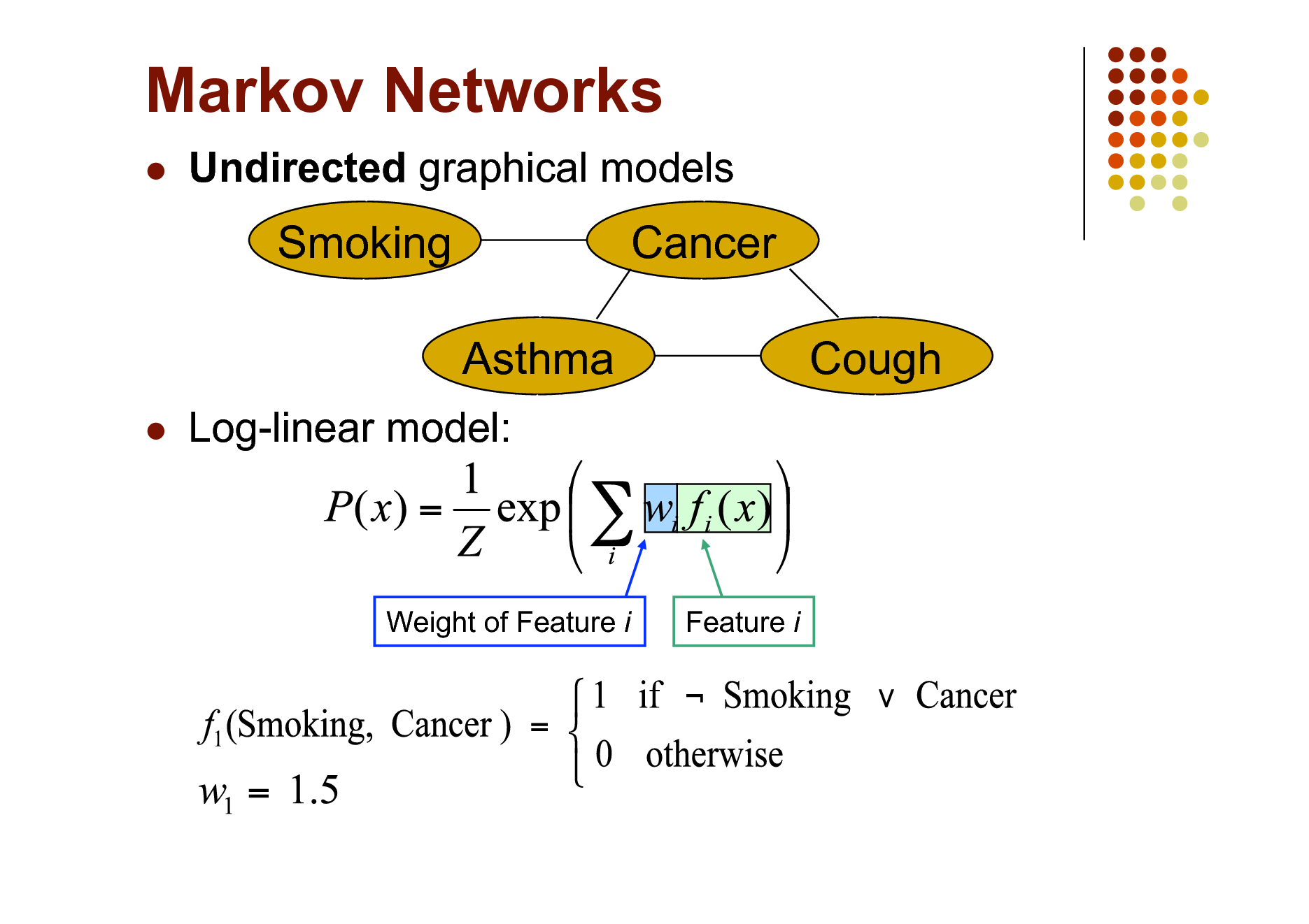
Markov Networks
Undirected graphical models
Smoking Asthma
Cancer Cough
Log-linear model:
Weight of Feature i
Feature i
11
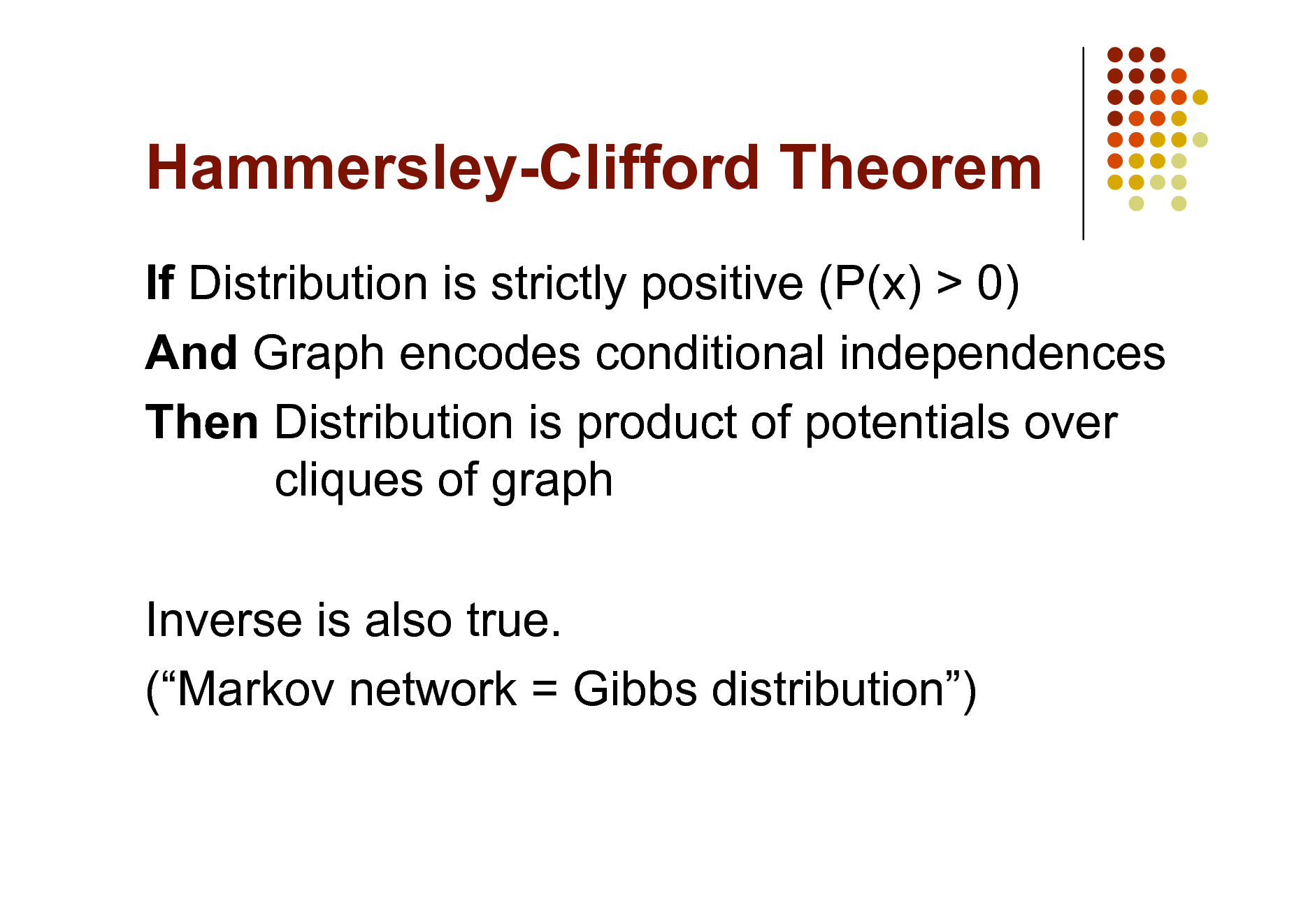
Hammersley-Clifford Theorem
If Distribution is strictly positive (P(x) > 0) And Graph encodes conditional independences Then Distribution is product of potentials over cliques of graph Inverse is also true. (Markov network = Gibbs distribution)
12
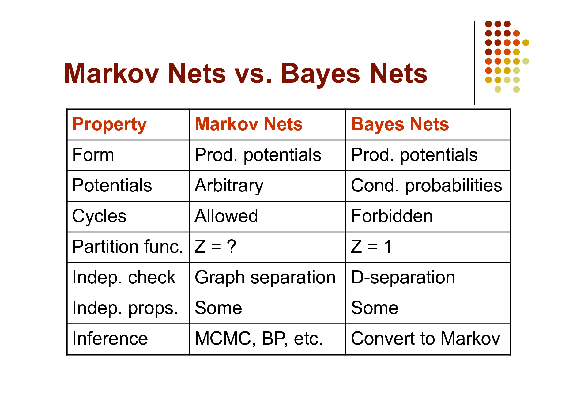
Markov Nets vs. Bayes Nets
Property Form Potentials Cycles Indep. check Inference Markov Nets Prod. potentials Arbitrary Allowed Bayes Nets Prod. potentials Cond. probabilities Forbidden Z=1 Some Convert to Markov
Partition func. Z = ? Indep. props. Some MCMC, BP, etc.
Graph separation D-separation
13
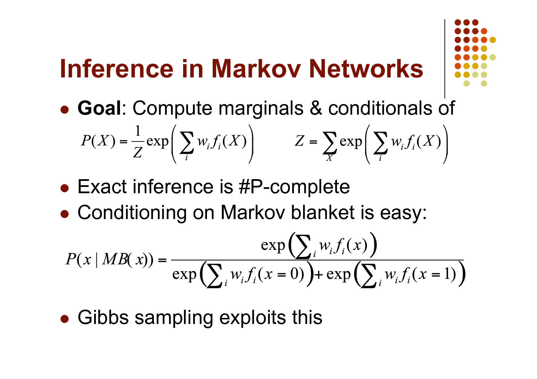
Inference in Markov Networks
Goal: Compute marginals & conditionals of
Exact inference is #P-complete Conditioning on Markov blanket is easy:
Gibbs sampling exploits this
14
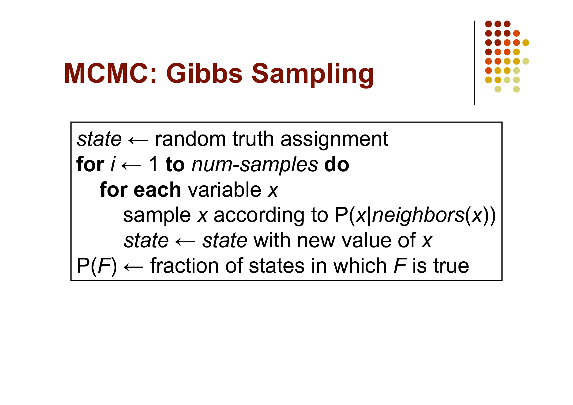
MCMC: Gibbs Sampling
state random truth assignment for i 1 to num-samples do for each variable x sample x according to P(x|neighbors(x)) state state with new value of x P(F) fraction of states in which F is true
15
Other Inference Methods
Many variations of MCMC Belief propagation (sum-product) Variational approximation Exact methods
16
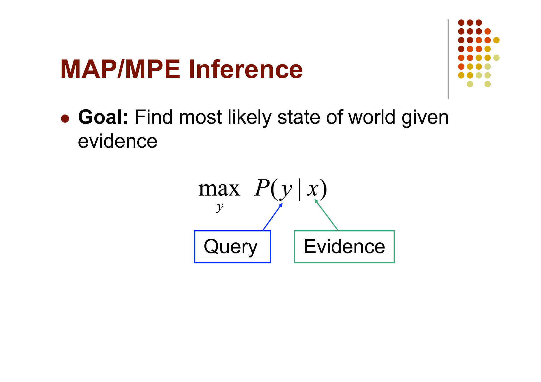
MAP/MPE Inference
Goal: Find most likely state of world given evidence
Query
Evidence
17
MAP Inference Algorithms
Iterated conditional modes Simulated annealing Graph cuts Belief propagation (max-product)
18
Overview
Motivation Foundational areas
Probabilistic inference Statistical learning Logical inference Inductive logic programming
Putting the pieces together Applications
19
Learning Markov Networks
Learning parameters (weights)
Generatively Discriminatively
Learning structure (features) In this tutorial: Assume complete data (If not: EM versions of algorithms)
20
Generative Weight Learning
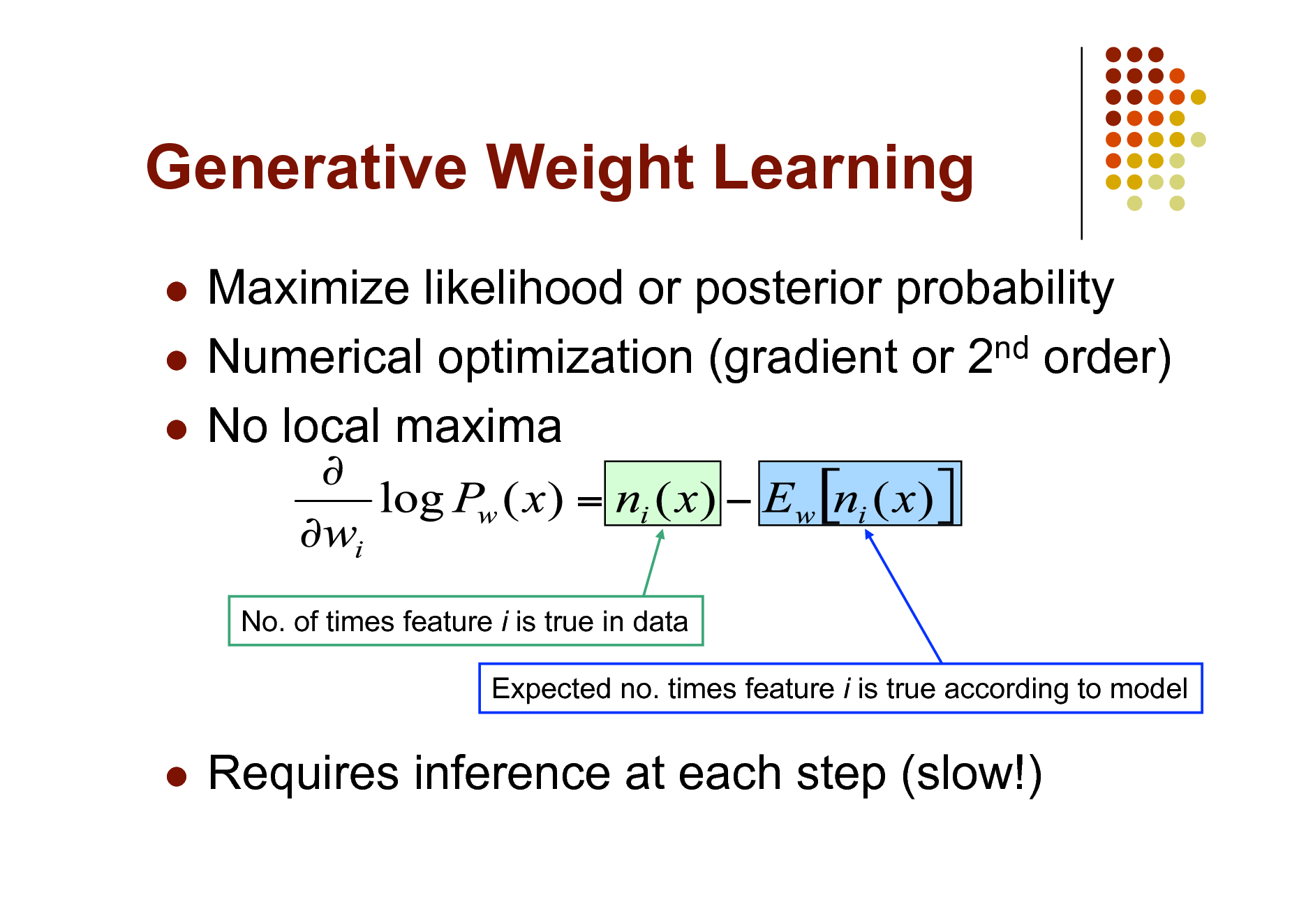
Maximize likelihood or posterior probability Numerical optimization (gradient or 2nd order) No local maxima
No. of times feature i is true in data Expected no. times feature i is true according to model
Requires inference at each step (slow!)
21
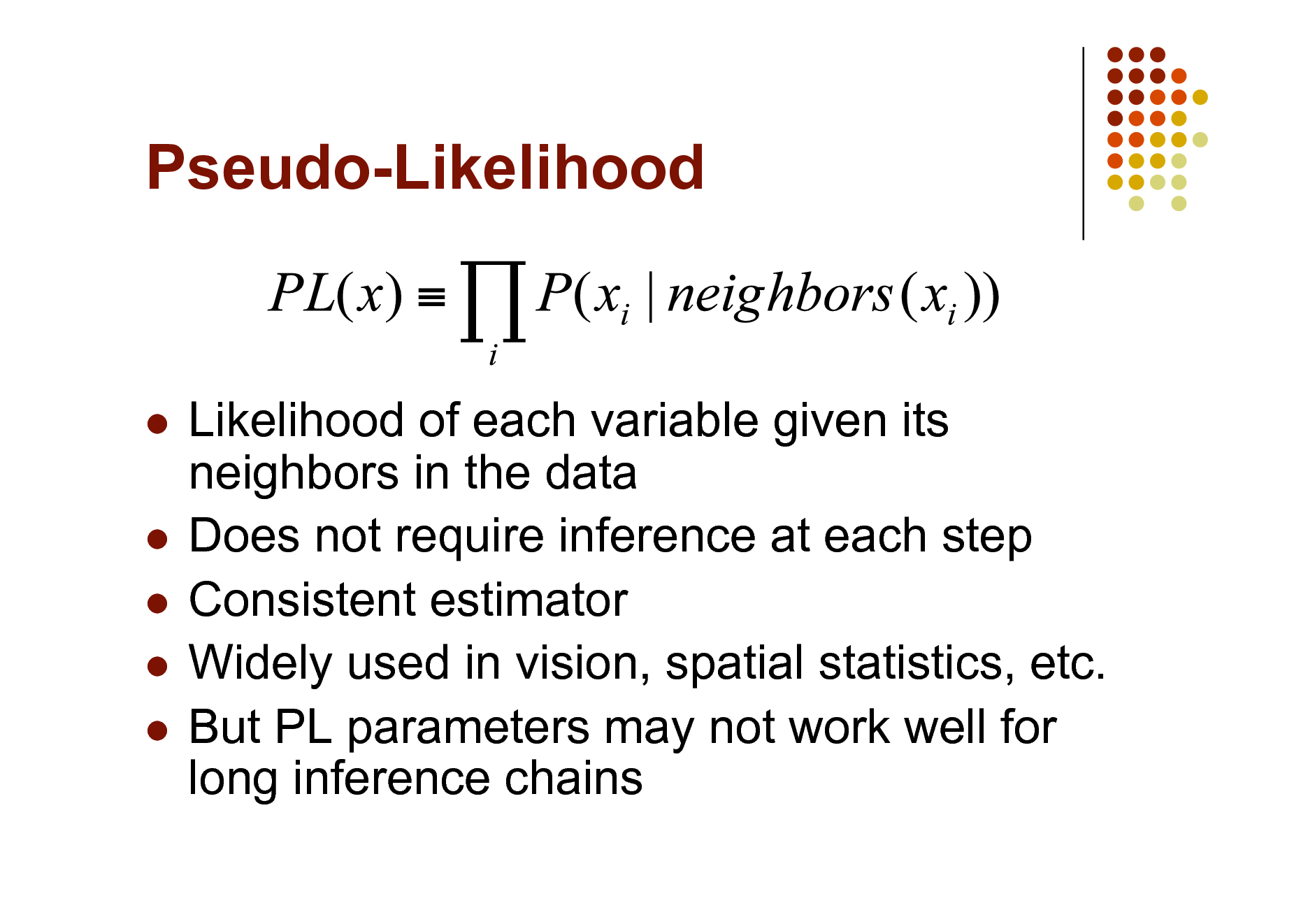
Pseudo-Likelihood
Likelihood of each variable given its neighbors in the data Does not require inference at each step Consistent estimator Widely used in vision, spatial statistics, etc. But PL parameters may not work well for long inference chains
22
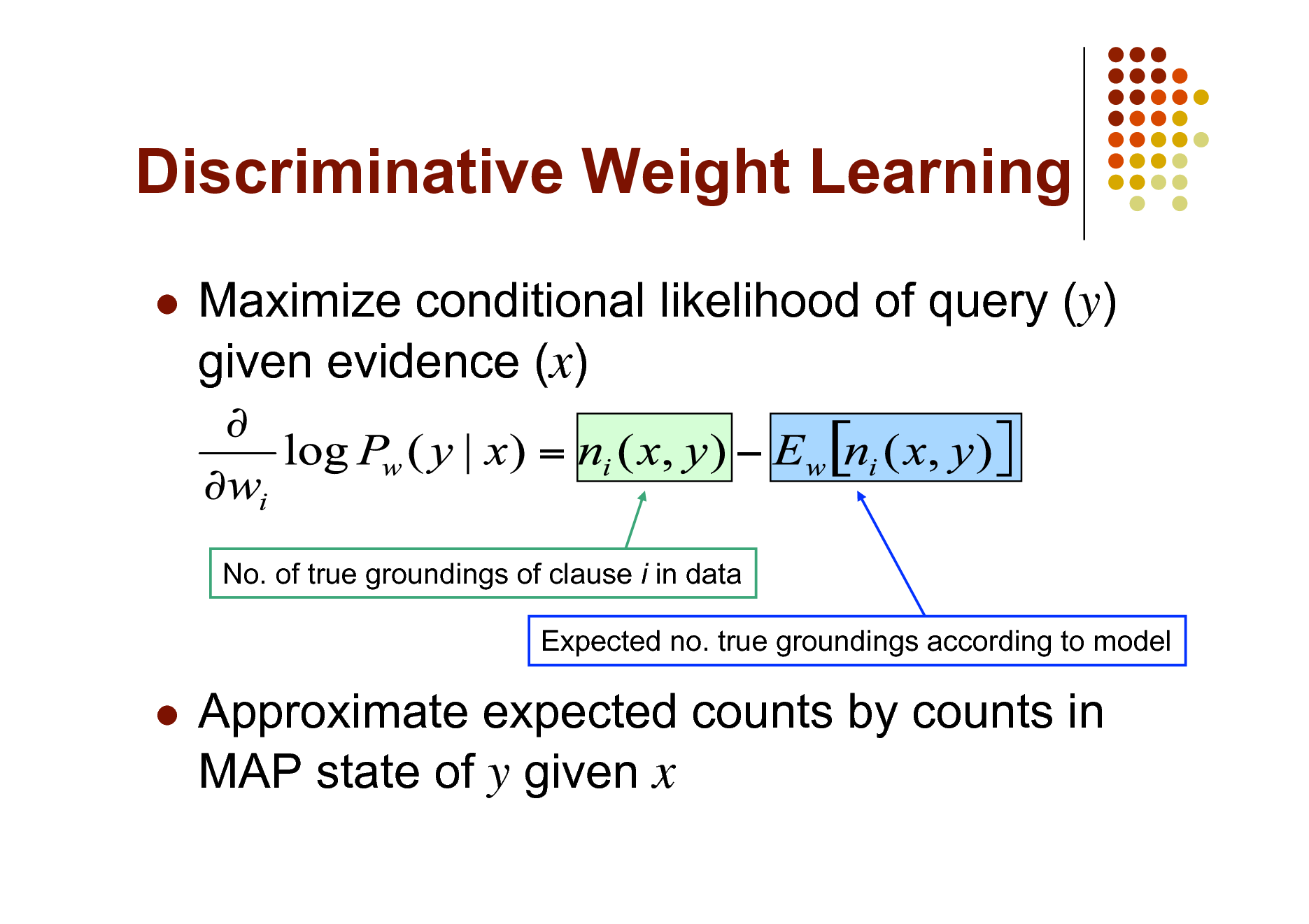
Discriminative Weight Learning
Maximize conditional likelihood of query (y) given evidence (x)
No. of true groundings of clause i in data Expected no. true groundings according to model
Approximate expected counts by counts in MAP state of y given x
23
Other Weight Learning Approaches
Generative: Iterative scaling Discriminative: Max margin
24
Structure Learning
Start with atomic features Greedily conjoin features to improve score Problem: Need to reestimate weights for each new candidate Approximation: Keep weights of previous features constant
25
Overview
Motivation Foundational areas
Probabilistic inference Statistical learning Logical inference Inductive logic programming
Putting the pieces together Applications
26
First-Order Logic
Constants, variables, functions, predicates E.g.: Anna, x, MotherOf(x), Friends(x, y) Literal: Predicate or its negation Clause: Disjunction of literals Grounding: Replace all variables by constants E.g.: Friends (Anna, Bob) World (model, interpretation): Assignment of truth values to all ground predicates
27
Inference in First-Order Logic
Traditionally done by theorem proving (e.g.: Prolog) Propositionalization followed by model checking turns out to be faster (often a lot) Propositionalization: Create all ground atoms and clauses Model checking: Satisfiability testing Two main approaches:
Backtracking (e.g.: DPLL) Stochastic local search (e.g.: WalkSAT)
28
Satisfiability
Input: Set of clauses (Convert KB to conjunctive normal form (CNF)) Output: Truth assignment that satisfies all clauses, or failure The paradigmatic NP-complete problem Solution: Search Key point: Most SAT problems are actually easy Hard region: Narrow range of #Clauses / #Variables
29
Backtracking
Assign truth values by depth-first search Assigning a variable deletes false literals and satisfied clauses Empty set of clauses: Success Empty clause: Failure Additional improvements:
Unit propagation (unit clause forces truth value) Pure literals (same truth value everywhere)
30
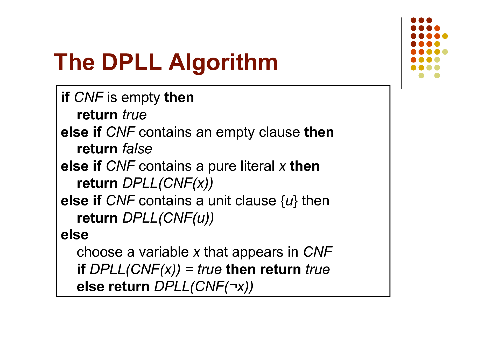
The DPLL Algorithm
if CNF is empty then return true else if CNF contains an empty clause then return false else if CNF contains a pure literal x then return DPLL(CNF(x)) else if CNF contains a unit clause {u} then return DPLL(CNF(u)) else choose a variable x that appears in CNF if DPLL(CNF(x)) = true then return true else return DPLL(CNF(x))
31
Stochastic Local Search
Uses complete assignments instead of partial Start with random state Flip variables in unsatisfied clauses Hill-climbing: Minimize # unsatisfied clauses Avoid local minima: Random flips Multiple restarts
32
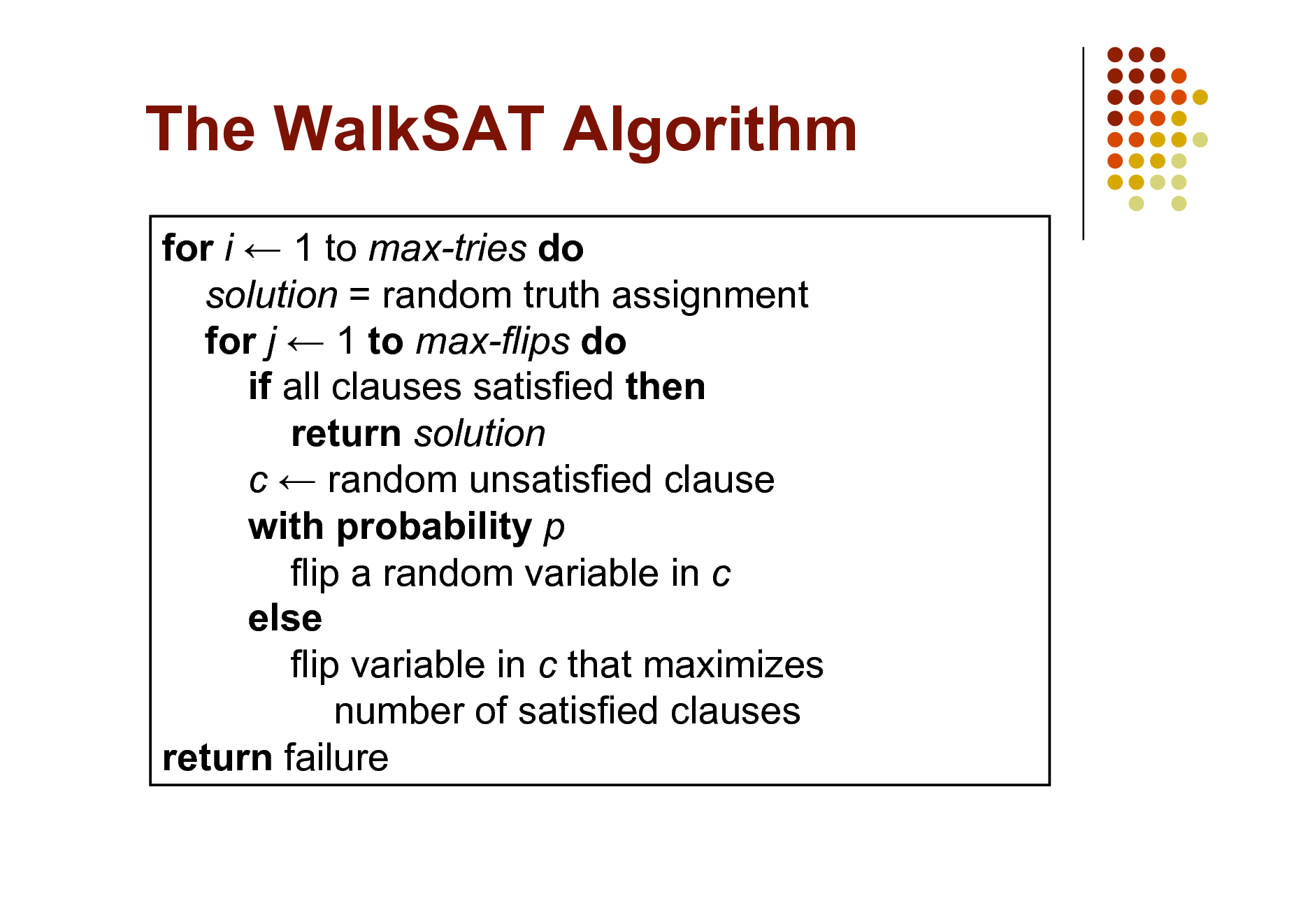
The WalkSAT Algorithm
for i 1 to max-tries do solution = random truth assignment for j 1 to max-flips do if all clauses satisfied then return solution c random unsatisfied clause with probability p flip a random variable in c else flip variable in c that maximizes number of satisfied clauses return failure
33
Overview
Motivation Foundational areas
Probabilistic inference Statistical learning Logical inference Inductive logic programming
Putting the pieces together Applications
34
Rule Induction
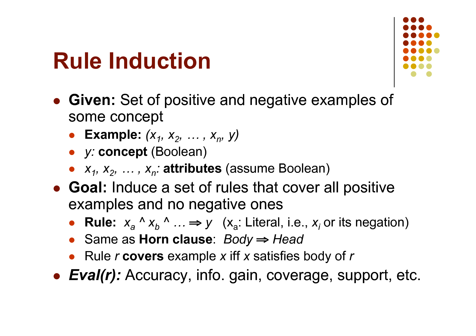
Given: Set of positive and negative examples of some concept
Example: (x1, x2, , xn, y) y: concept (Boolean) x1, x2, , xn: attributes (assume Boolean)
Goal: Induce a set of rules that cover all positive examples and no negative ones
Rule: xa ^ xb ^ y (xa: Literal, i.e., xi or its negation) Same as Horn clause: Body Head Rule r covers example x iff x satisfies body of r
Eval(r): Accuracy, info. gain, coverage, support, etc.
35
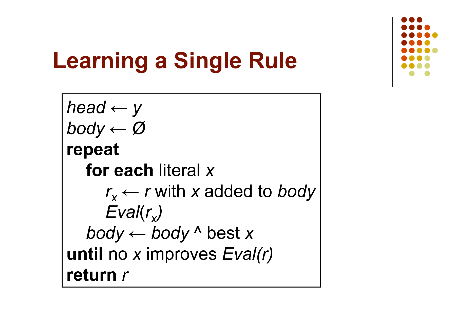
Learning a Single Rule
head y body repeat for each literal x rx r with x added to body Eval(rx) body body ^ best x until no x improves Eval(r) return r
36
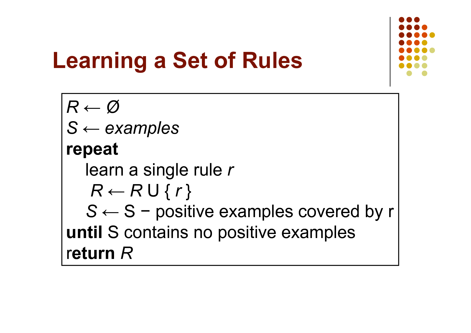
Learning a Set of Rules
R S examples repeat learn a single rule r RRU{r} S S positive examples covered by r until S contains no positive examples return R
37
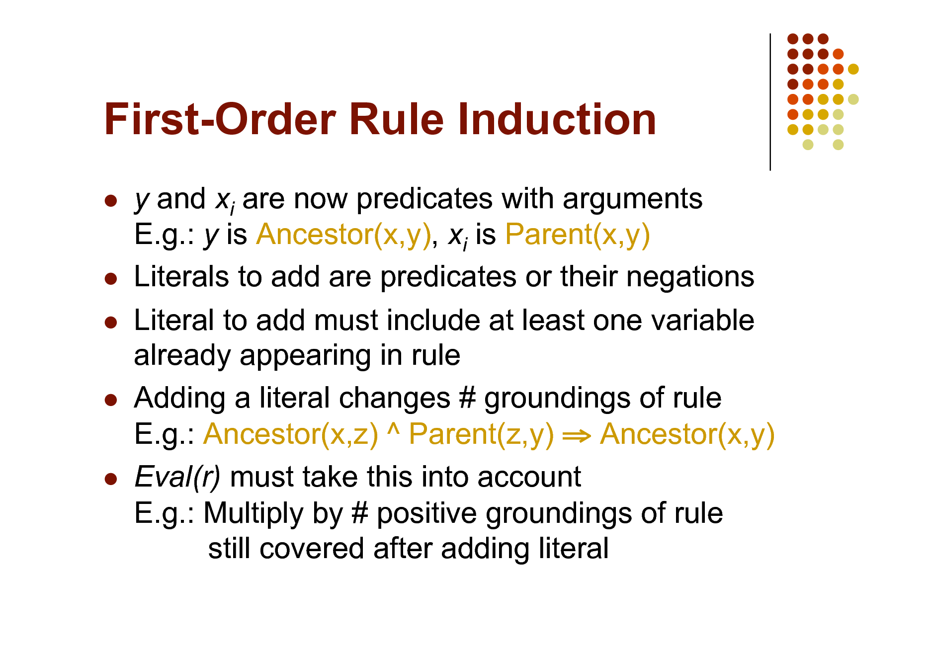
First-Order Rule Induction
y and xi are now predicates with arguments E.g.: y is Ancestor(x,y), xi is Parent(x,y) Literals to add are predicates or their negations Literal to add must include at least one variable already appearing in rule Adding a literal changes # groundings of rule E.g.: Ancestor(x,z) ^ Parent(z,y) Ancestor(x,y) Eval(r) must take this into account E.g.: Multiply by # positive groundings of rule still covered after adding literal
38
Overview
Motivation Foundational areas
Probabilistic inference Statistical learning Logical inference Inductive logic programming
Putting the pieces together Applications
39
![Slide: Plethora of Approaches
Knowledge-based model construction
[Wellman et al., 1992]
Stochastic logic programs [Muggleton, 1996] Probabilistic relational models
[Friedman et al., 1999]
Relational Markov networks [Taskar et al., 2002] Bayesian logic [Milch et al., 2005] Markov logic [Richardson & Domingos, 2006]
And many others!](https://yosinski.com/mlss12/media/slides/MLSS-2012-Domingos-Statistical-Relational-Learning_040.png)
Plethora of Approaches
Knowledge-based model construction
[Wellman et al., 1992]
Stochastic logic programs [Muggleton, 1996] Probabilistic relational models
[Friedman et al., 1999]
Relational Markov networks [Taskar et al., 2002] Bayesian logic [Milch et al., 2005] Markov logic [Richardson & Domingos, 2006]
And many others!
40
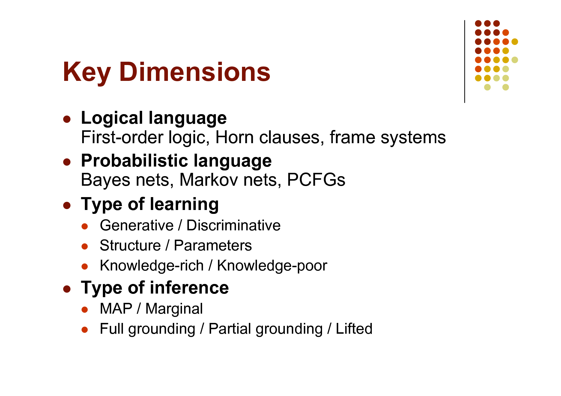
Key Dimensions
Logical language First-order logic, Horn clauses, frame systems Probabilistic language Bayes nets, Markov nets, PCFGs Type of learning
Generative / Discriminative Structure / Parameters Knowledge-rich / Knowledge-poor MAP / Marginal Full grounding / Partial grounding / Lifted
Type of inference
41
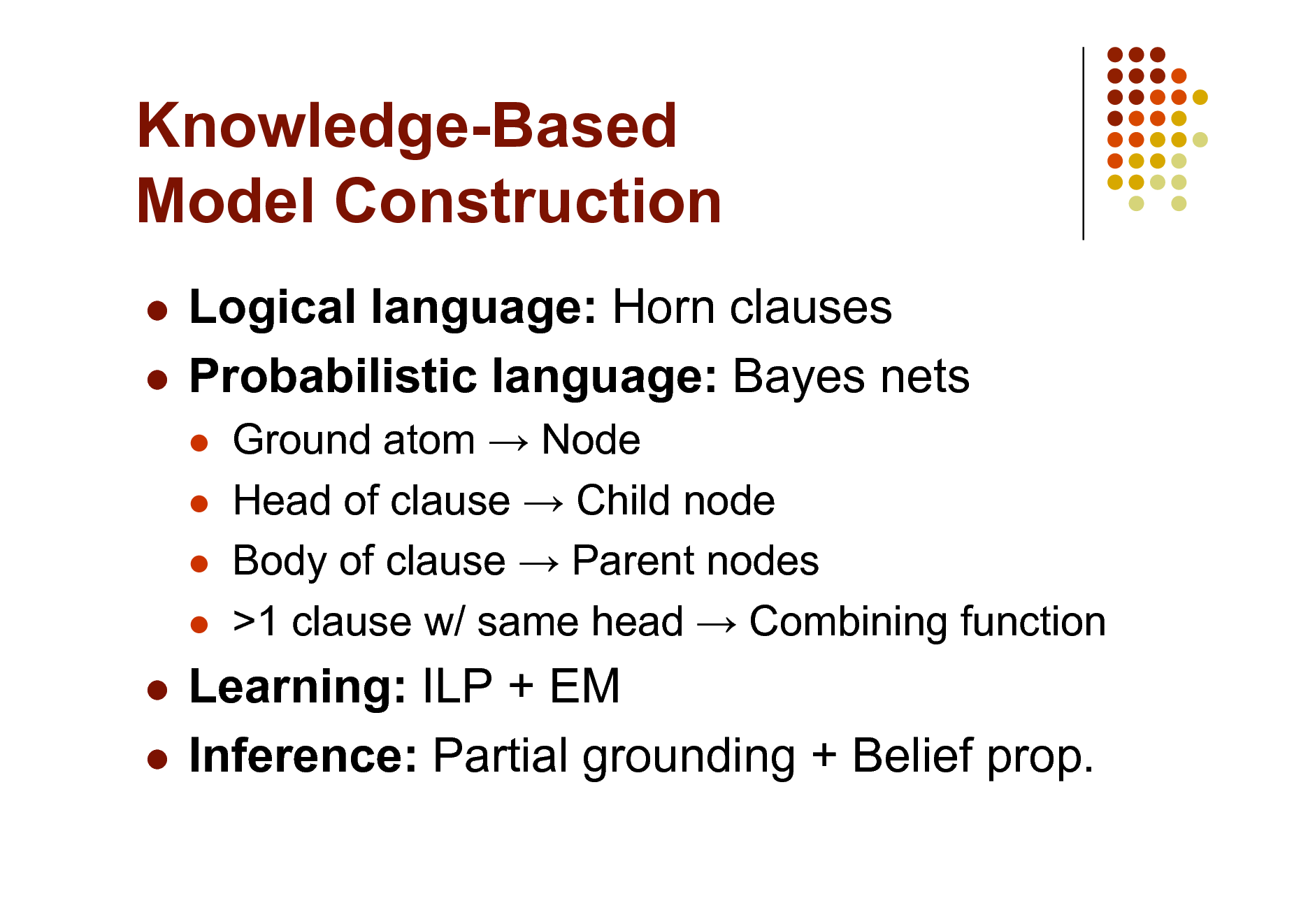
Knowledge-Based Model Construction
Logical language: Horn clauses Probabilistic language: Bayes nets
Ground atom Node Head of clause Child node Body of clause Parent nodes >1 clause w/ same head Combining function
Learning: ILP + EM Inference: Partial grounding + Belief prop.
42
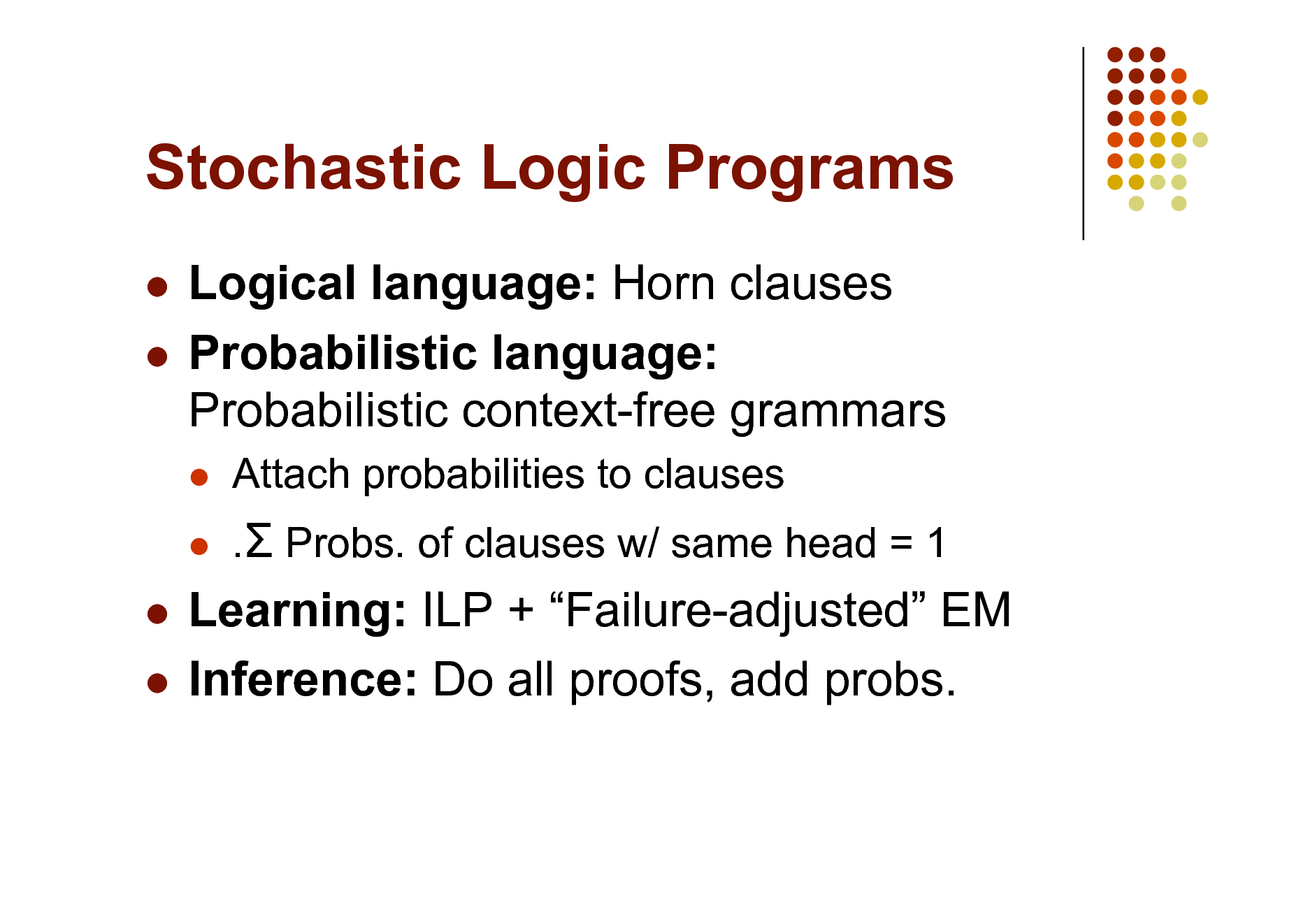
Stochastic Logic Programs
Logical language: Horn clauses Probabilistic language: Probabilistic context-free grammars
Attach probabilities to clauses . Probs. of clauses w/ same head = 1
Learning: ILP + Failure-adjusted EM Inference: Do all proofs, add probs.
43
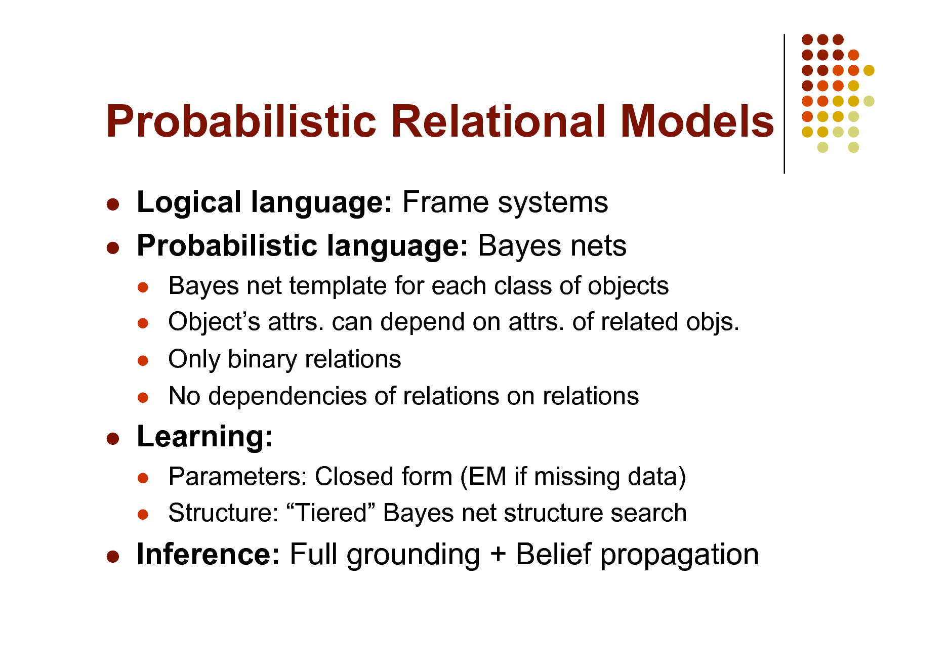
Probabilistic Relational Models
Logical language: Frame systems Probabilistic language: Bayes nets
Bayes net template for each class of objects Objects attrs. can depend on attrs. of related objs. Only binary relations No dependencies of relations on relations Parameters: Closed form (EM if missing data) Structure: Tiered Bayes net structure search
Learning:
Inference: Full grounding + Belief propagation
44
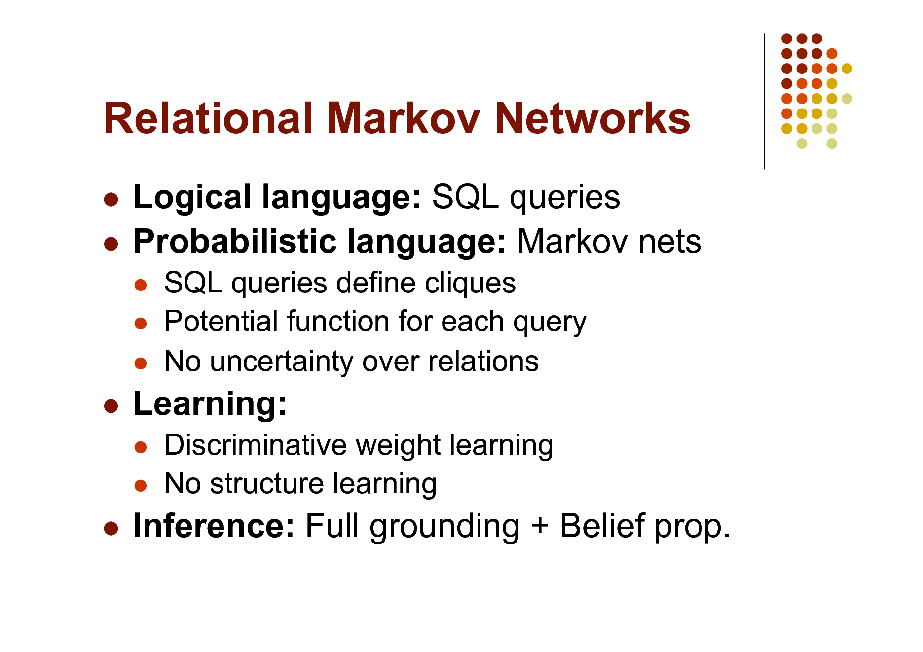
Relational Markov Networks
Logical language: SQL queries Probabilistic language: Markov nets
SQL queries define cliques Potential function for each query No uncertainty over relations Discriminative weight learning No structure learning
Learning:
Inference: Full grounding + Belief prop.
45
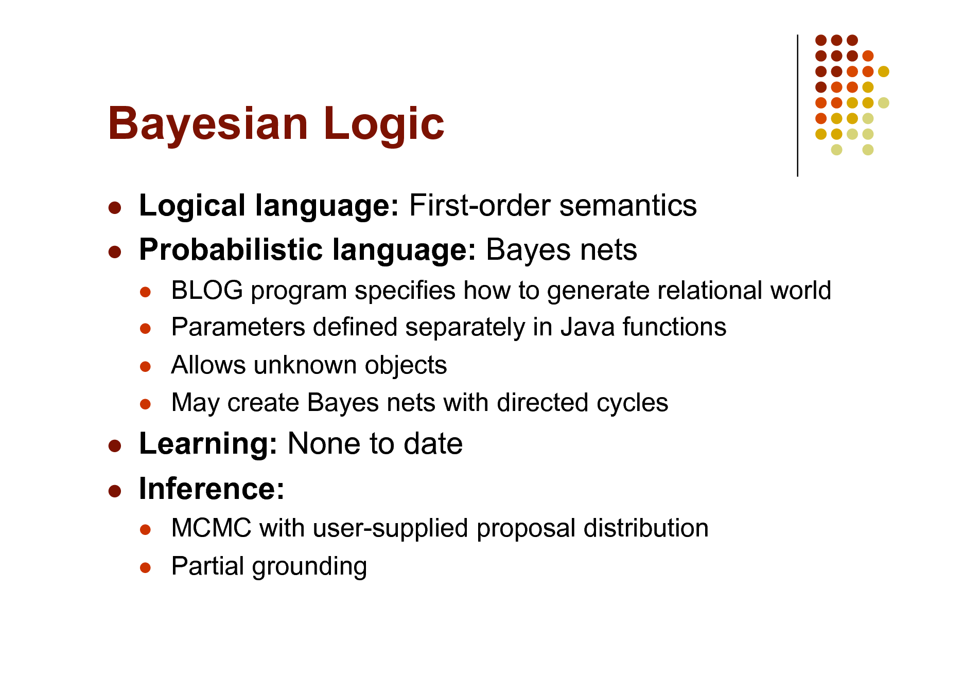
Bayesian Logic
Logical language: First-order semantics Probabilistic language: Bayes nets
BLOG program specifies how to generate relational world Parameters defined separately in Java functions Allows unknown objects May create Bayes nets with directed cycles
Learning: None to date Inference:
MCMC with user-supplied proposal distribution Partial grounding
46
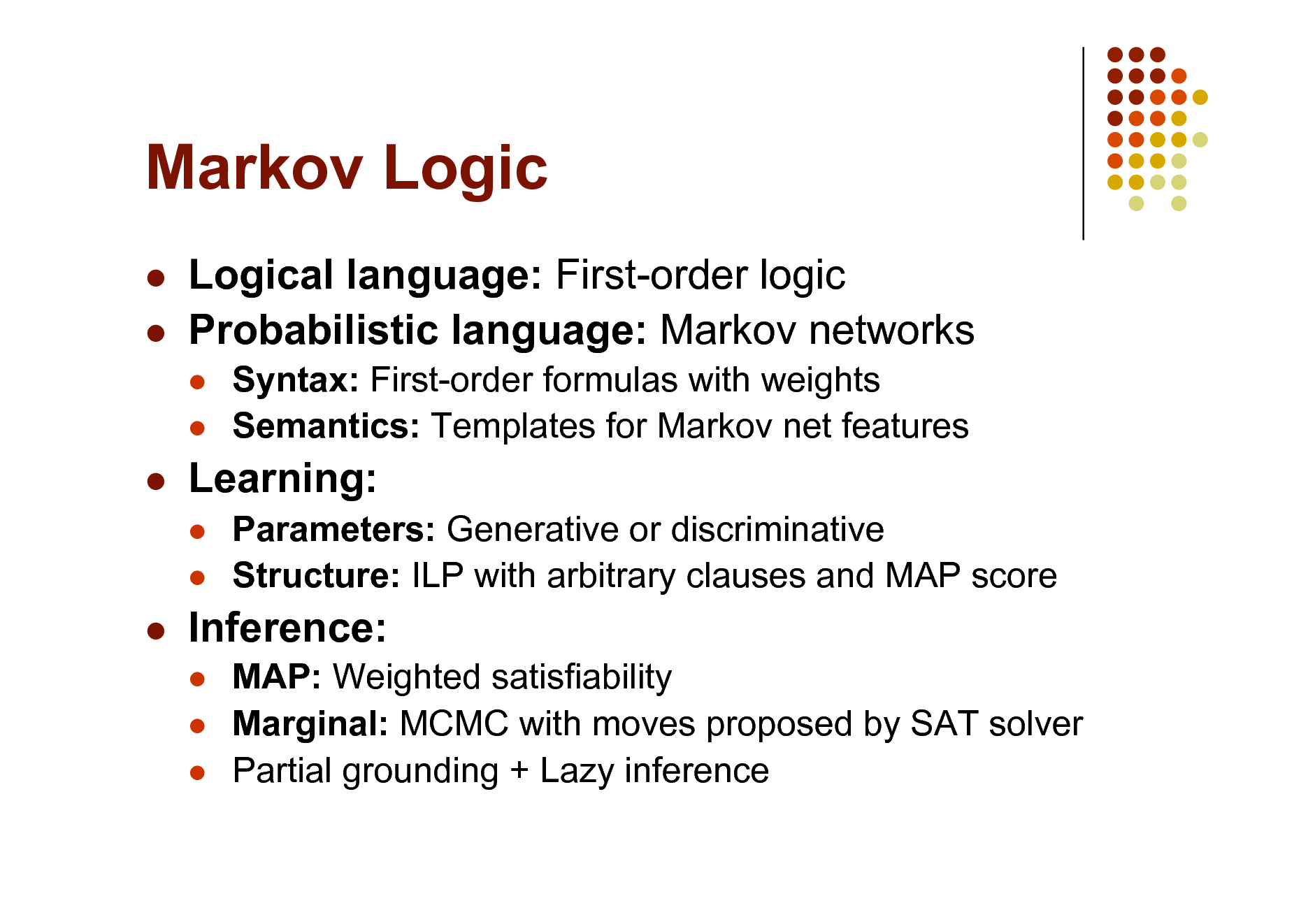
Markov Logic
Logical language: First-order logic Probabilistic language: Markov networks
Syntax: First-order formulas with weights Semantics: Templates for Markov net features Parameters: Generative or discriminative Structure: ILP with arbitrary clauses and MAP score MAP: Weighted satisfiability Marginal: MCMC with moves proposed by SAT solver Partial grounding + Lazy inference
Learning:
Inference:
47
Markov Logic
Most developed approach to date Many other approaches can be viewed as special cases Main focus of rest of this tutorial
48
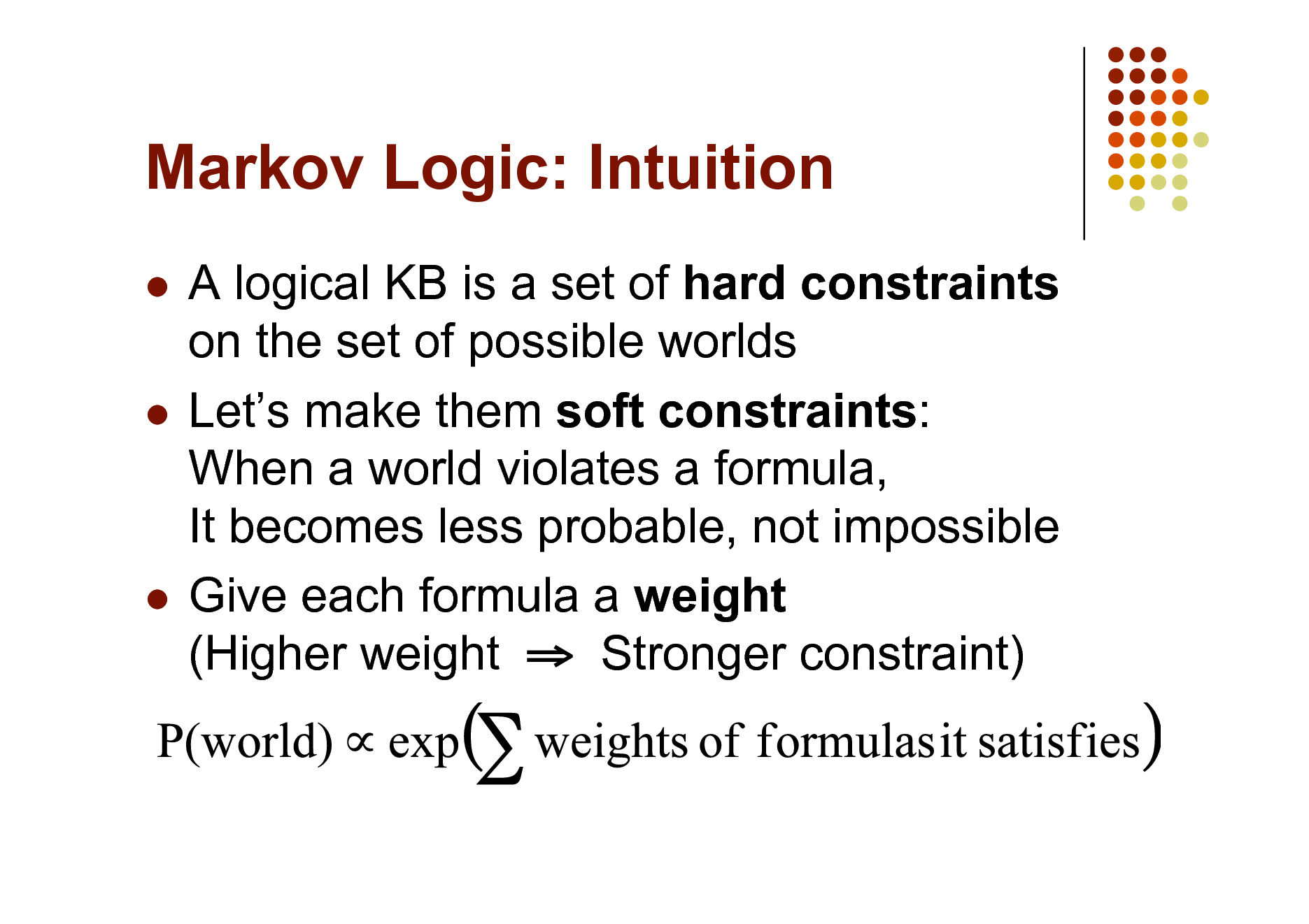
Markov Logic: Intuition
A logical KB is a set of hard constraints on the set of possible worlds Lets make them soft constraints: When a world violates a formula, It becomes less probable, not impossible Give each formula a weight (Higher weight Stronger constraint)
49
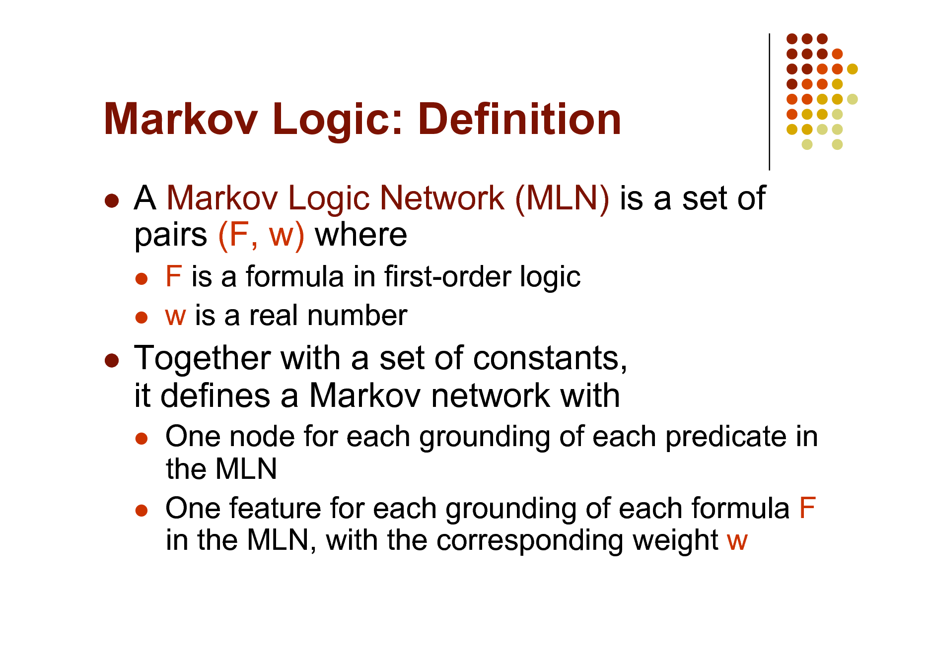
Markov Logic: Definition
A Markov Logic Network (MLN) is a set of pairs (F, w) where
F is a formula in first-order logic w is a real number
Together with a set of constants, it defines a Markov network with
One node for each grounding of each predicate in the MLN One feature for each grounding of each formula F in the MLN, with the corresponding weight w
50
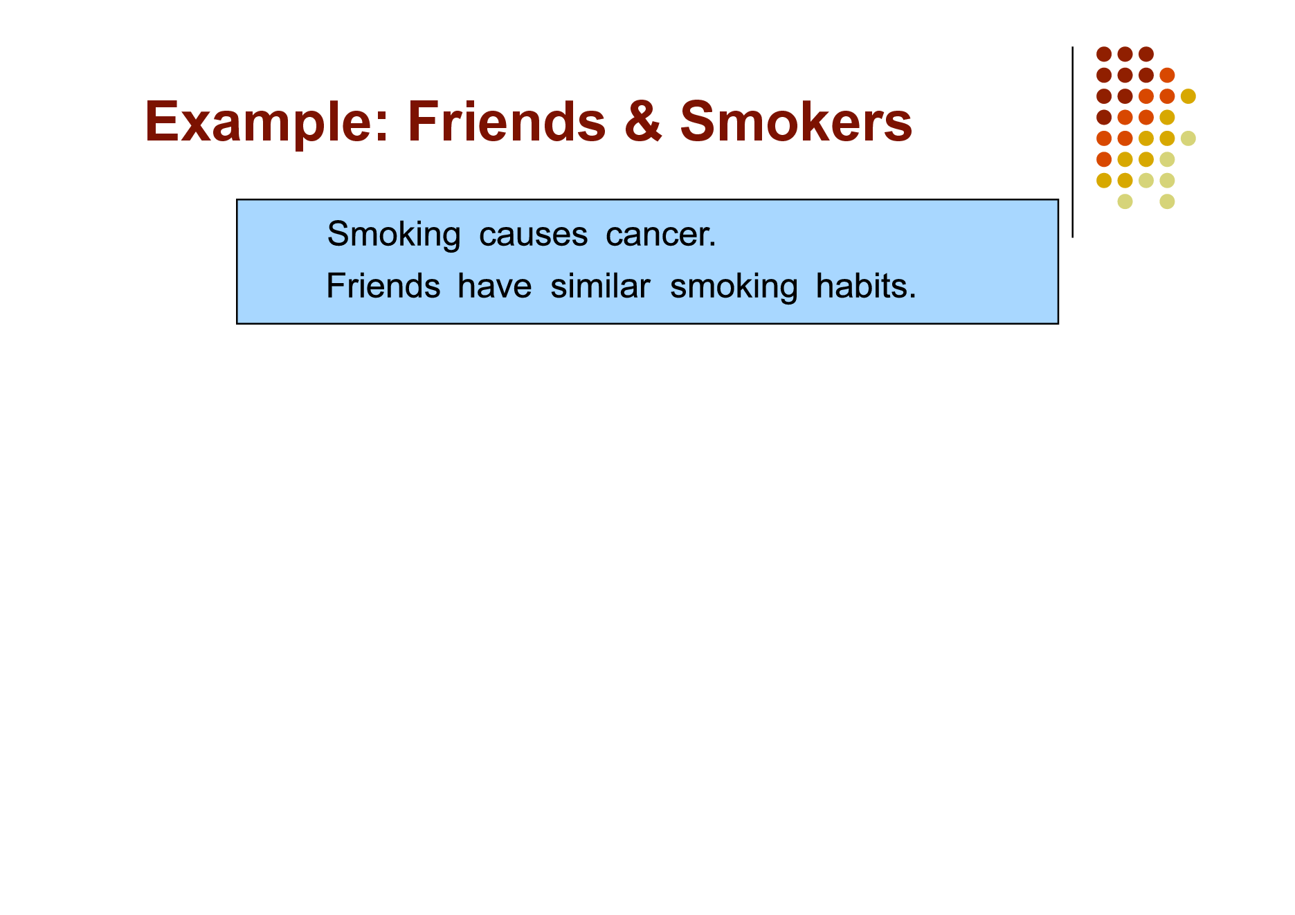
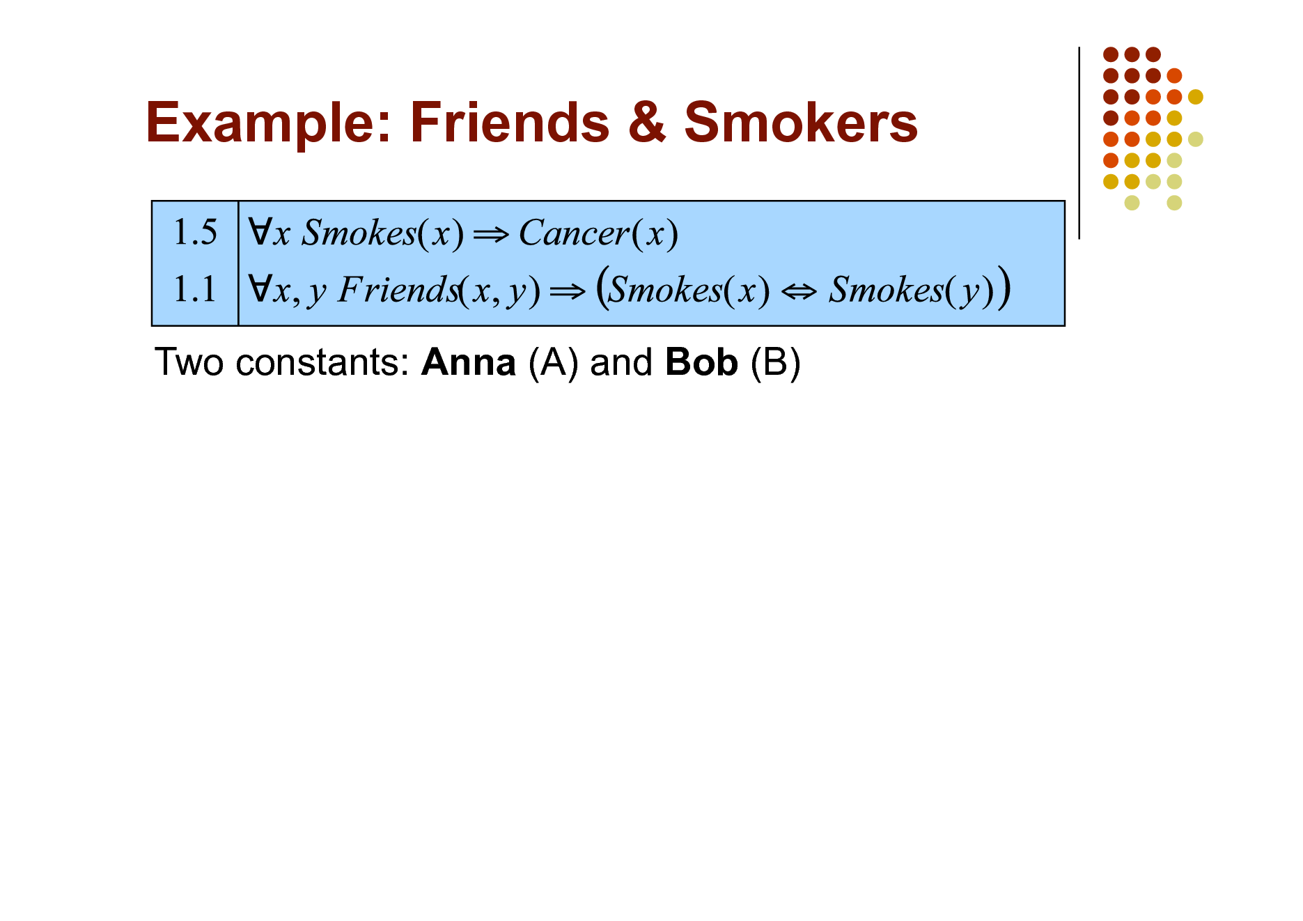
Example: Friends & Smokers
51
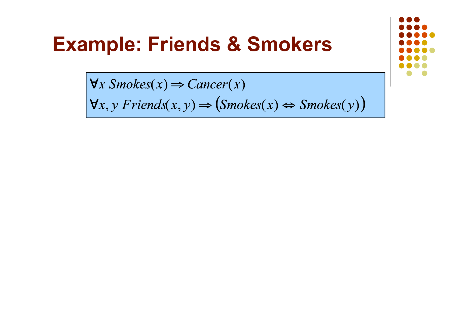
Example: Friends & Smokers
52
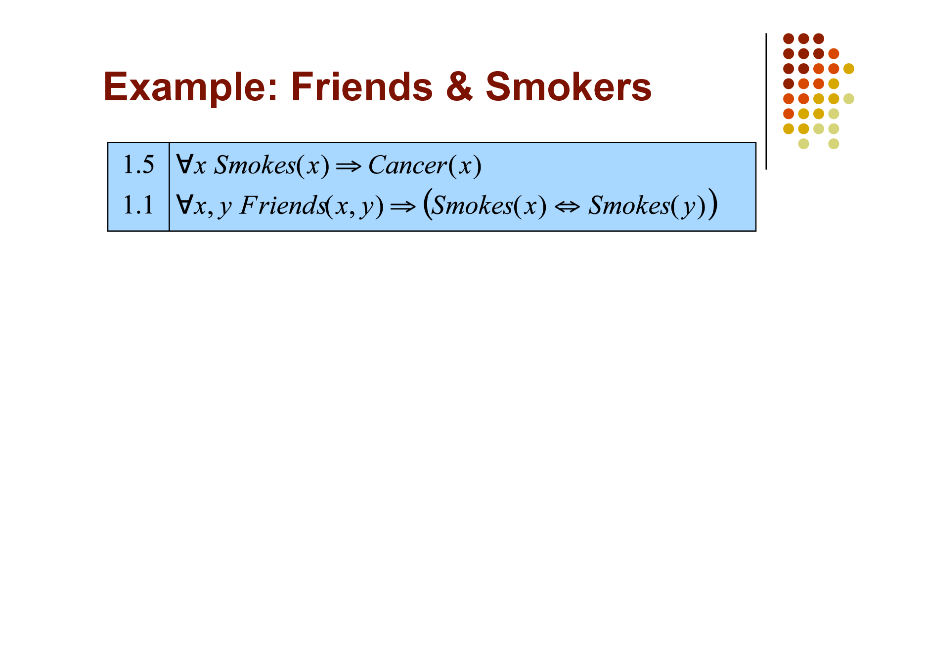
Example: Friends & Smokers
53
Example: Friends & Smokers
Two constants: Anna (A) and Bob (B)
54
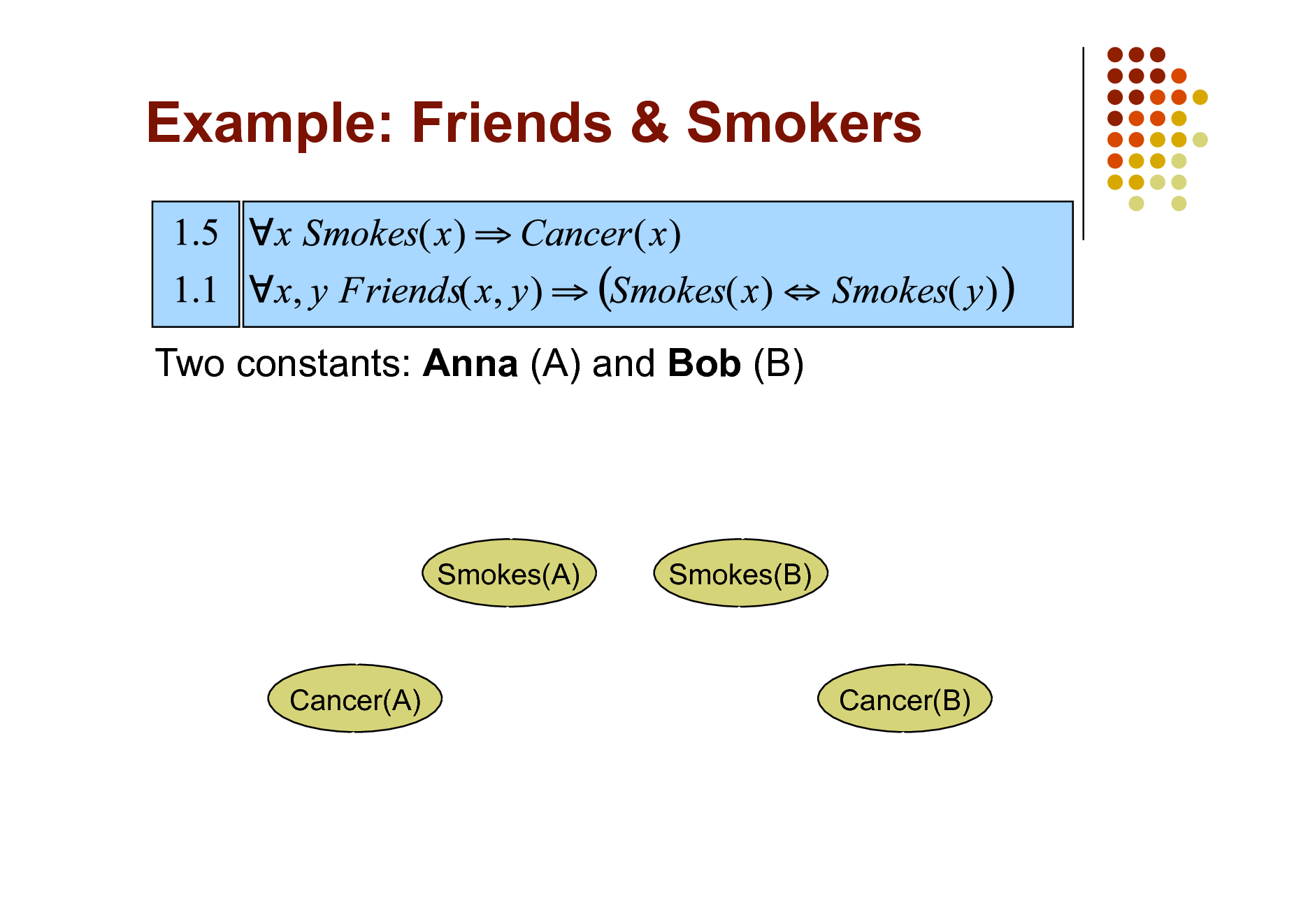
Example: Friends & Smokers
Two constants: Anna (A) and Bob (B)
Smokes(A)
Smokes(B)
Cancer(A)
Cancer(B)
55

Example: Friends & Smokers
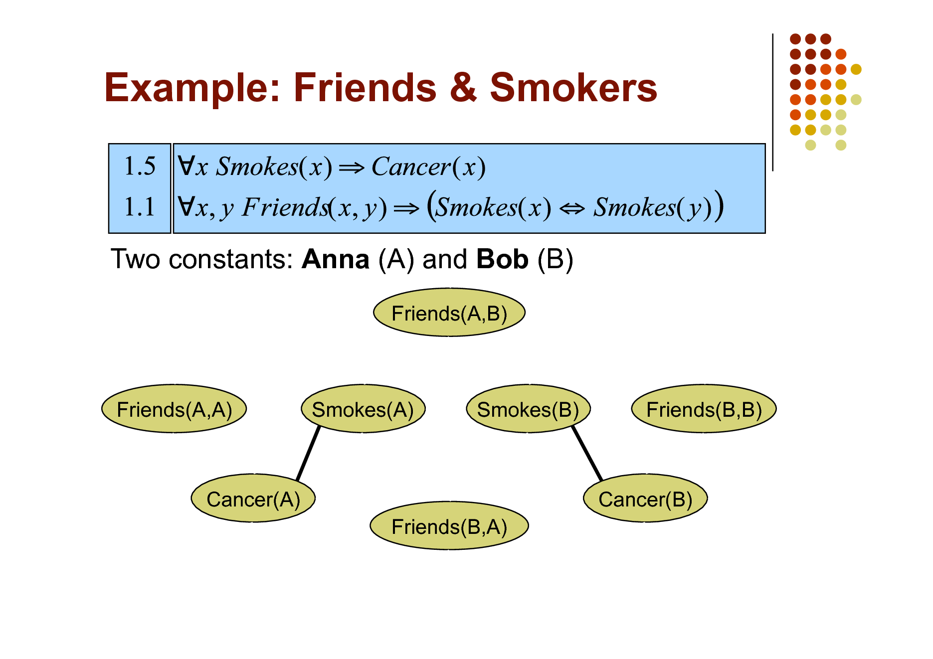
Two constants: Anna (A) and Bob (B)
Friends(A,B)
Friends(A,A)
Smokes(A)
Smokes(B)
Friends(B,B)
Cancer(A) Friends(B,A)
Cancer(B)
56
Example: Friends & Smokers
Two constants: Anna (A) and Bob (B)
Friends(A,B)
Friends(A,A)
Smokes(A)
Smokes(B)
Friends(B,B)
Cancer(A) Friends(B,A)
Cancer(B)
57

Example: Friends & Smokers
Two constants: Anna (A) and Bob (B)
Friends(A,B)
Friends(A,A)
Smokes(A)
Smokes(B)
Friends(B,B)
Cancer(A) Friends(B,A)
Cancer(B)
58
Markov Logic Networks
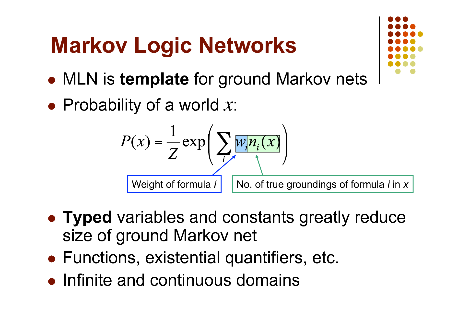
MLN is template for ground Markov nets Probability of a world x:
Weight of formula i
No. of true groundings of formula i in x
Typed variables and constants greatly reduce size of ground Markov net Functions, existential quantifiers, etc. Infinite and continuous domains
59
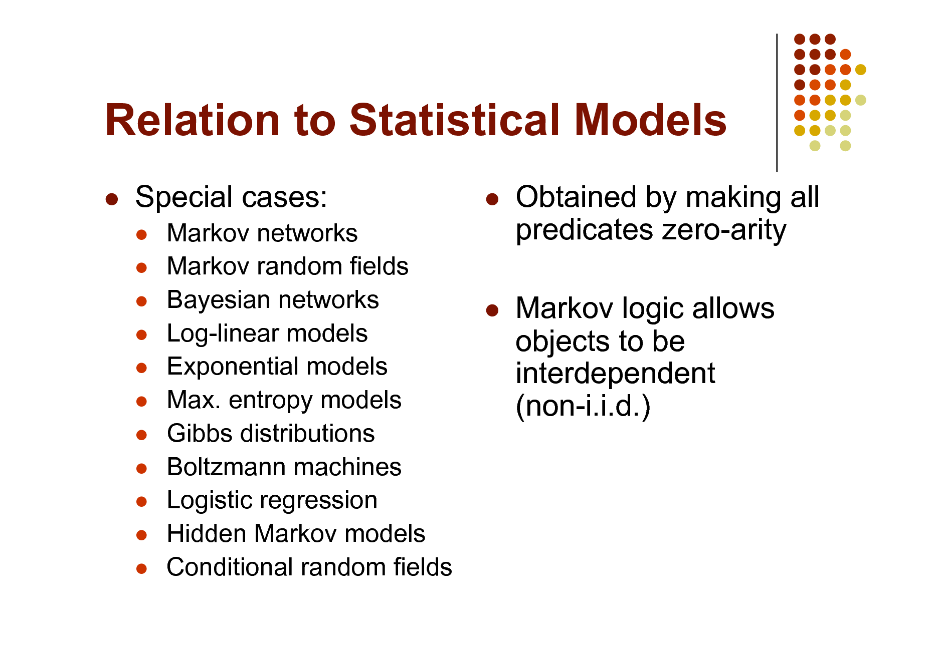
Relation to Statistical Models
Special cases:
Markov networks Markov random fields Bayesian networks Log-linear models Exponential models Max. entropy models Gibbs distributions Boltzmann machines Logistic regression Hidden Markov models Conditional random fields
Obtained by making all predicates zero-arity Markov logic allows objects to be interdependent (non-i.i.d.)
60

Relation to First-Order Logic
Infinite weights First-order logic Satisfiable KB, positive weights Satisfying assignments = Modes of distribution Markov logic allows contradictions between formulas
61
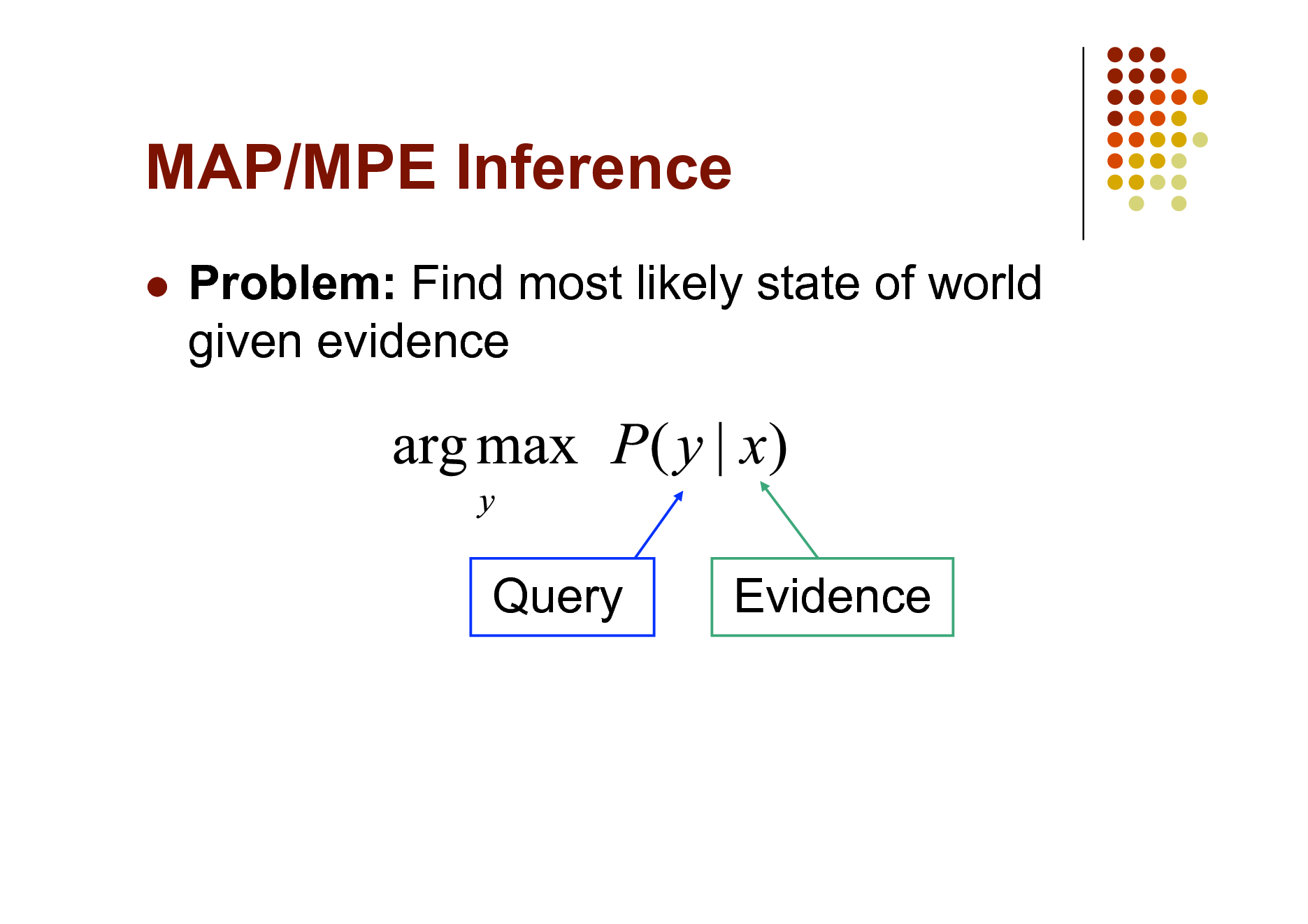
MAP/MPE Inference
Problem: Find most likely state of world given evidence
Query
Evidence
62
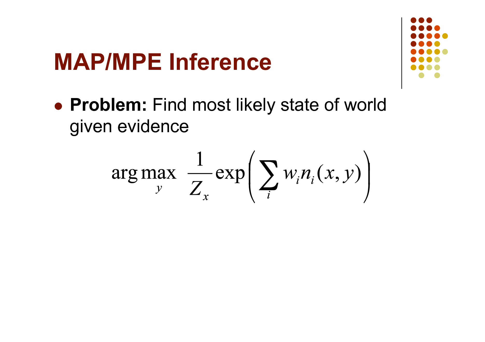
MAP/MPE Inference
Problem: Find most likely state of world given evidence
63
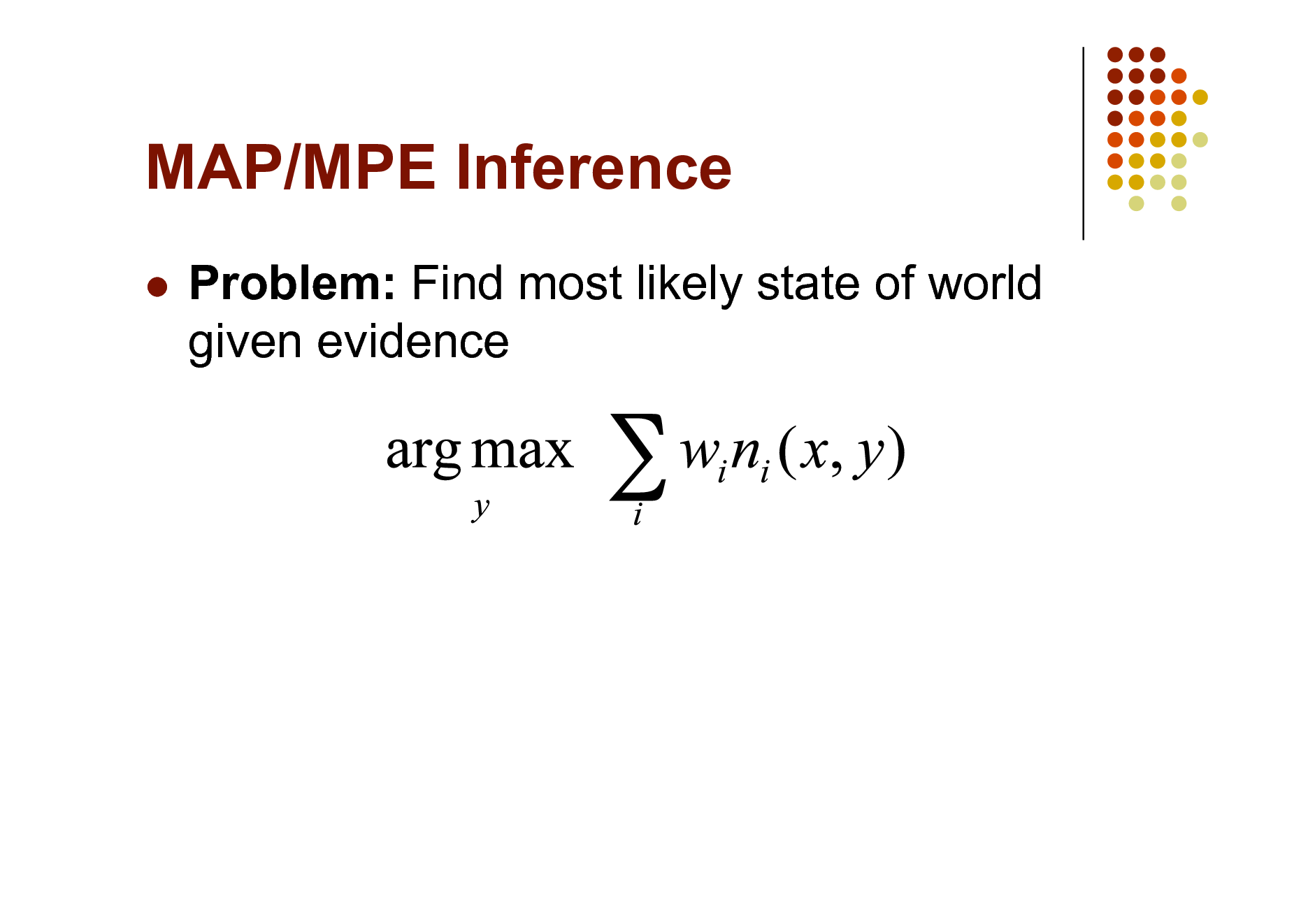
MAP/MPE Inference
Problem: Find most likely state of world given evidence
64
![Slide: MAP/MPE Inference
Problem: Find most likely state of world given evidence
This is just the weighted MaxSAT problem Use weighted SAT solver (e.g., MaxWalkSAT [Kautz et al., 1997] ) Potentially faster than logical inference (!)](https://yosinski.com/mlss12/media/slides/MLSS-2012-Domingos-Statistical-Relational-Learning_065.png)
MAP/MPE Inference
Problem: Find most likely state of world given evidence
This is just the weighted MaxSAT problem Use weighted SAT solver (e.g., MaxWalkSAT [Kautz et al., 1997] ) Potentially faster than logical inference (!)
65
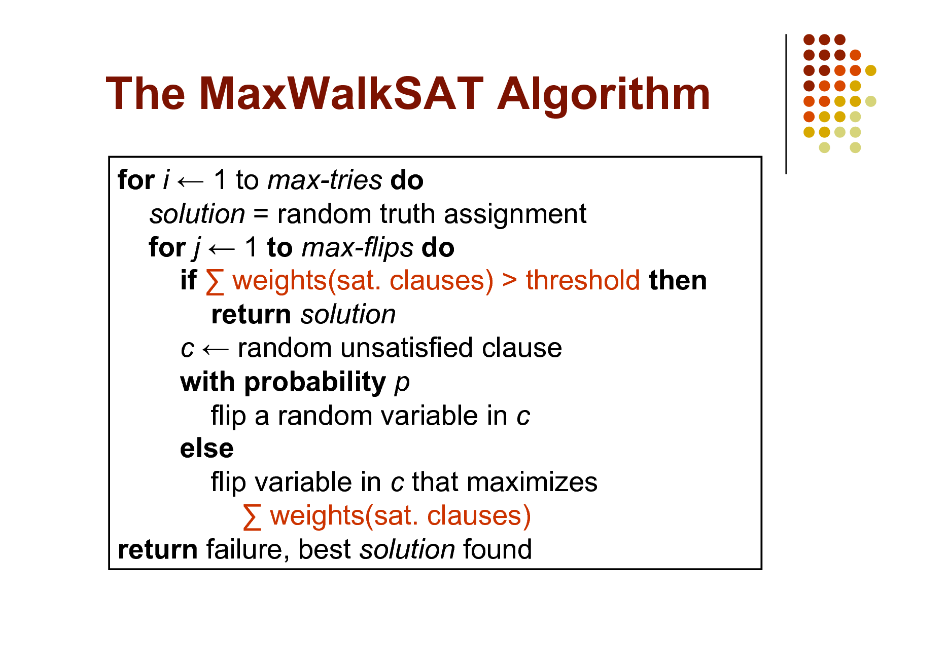
The MaxWalkSAT Algorithm
for i 1 to max-tries do solution = random truth assignment for j 1 to max-flips do if weights(sat. clauses) > threshold then return solution c random unsatisfied clause with probability p flip a random variable in c else flip variable in c that maximizes weights(sat. clauses) return failure, best solution found
66
![Slide: But Memory Explosion
Problem: If there are n constants and the highest clause arity is c, c the ground network requires O(n ) memory Solution: Exploit sparseness; ground clauses lazily LazySAT algorithm [Singla & Domingos, 2006]](https://yosinski.com/mlss12/media/slides/MLSS-2012-Domingos-Statistical-Relational-Learning_067.png)
But Memory Explosion
Problem: If there are n constants and the highest clause arity is c, c the ground network requires O(n ) memory Solution: Exploit sparseness; ground clauses lazily LazySAT algorithm [Singla & Domingos, 2006]
67
![Slide: Computing Probabilities
P(Formula|MLN,C) = ? MCMC: Sample worlds, check formula holds P(Formula1|Formula2,MLN,C) = ? If Formula2 = Conjunction of ground atoms
First construct min subset of network necessary to answer query (generalization of KBMC) Then apply MCMC (or other)
Can also do lifted inference [Braz et al, 2005]](https://yosinski.com/mlss12/media/slides/MLSS-2012-Domingos-Statistical-Relational-Learning_068.png)
Computing Probabilities
P(Formula|MLN,C) = ? MCMC: Sample worlds, check formula holds P(Formula1|Formula2,MLN,C) = ? If Formula2 = Conjunction of ground atoms
First construct min subset of network necessary to answer query (generalization of KBMC) Then apply MCMC (or other)
Can also do lifted inference [Braz et al, 2005]
68
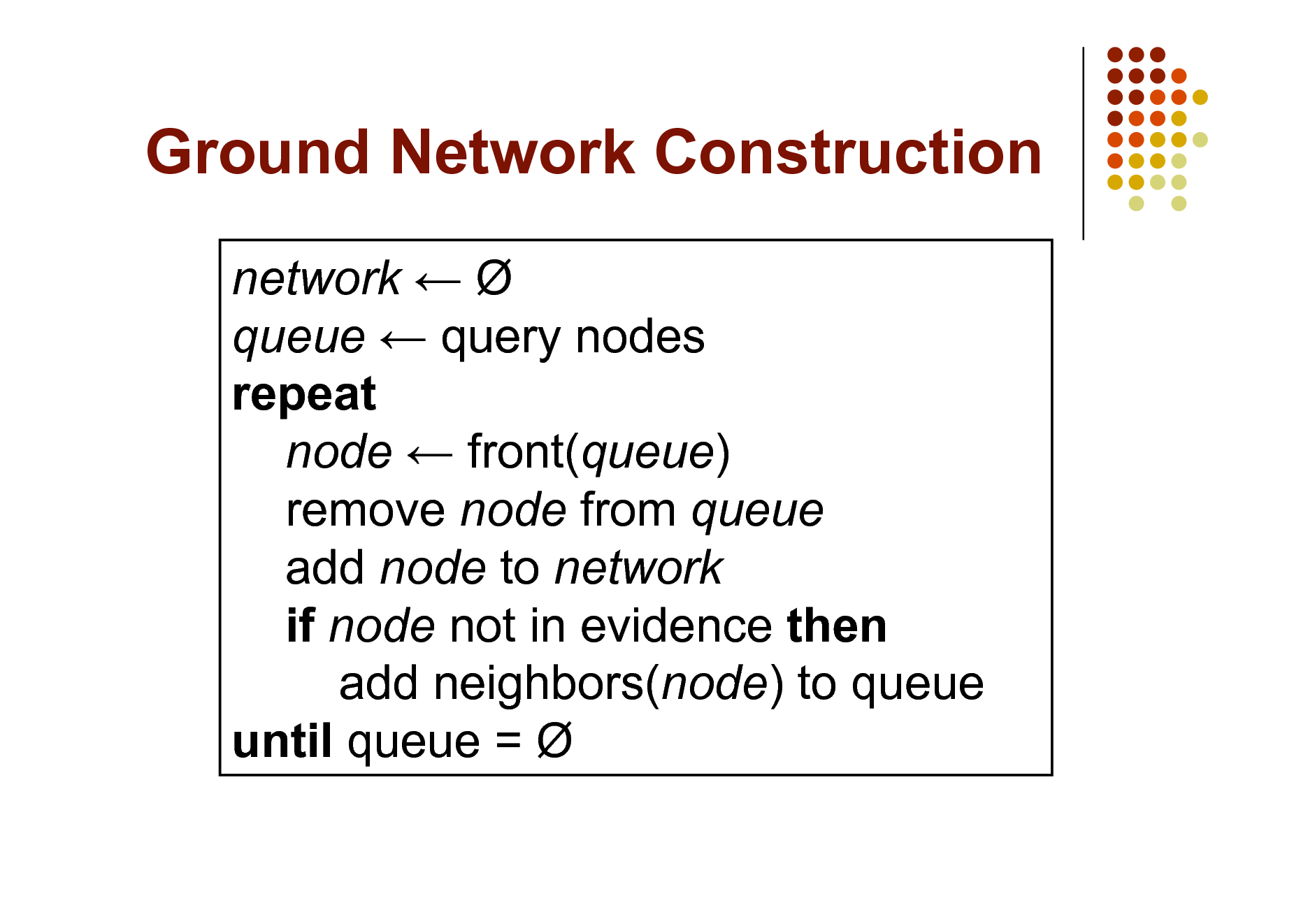
Ground Network Construction
network queue query nodes repeat node front(queue) remove node from queue add node to network if node not in evidence then add neighbors(node) to queue until queue =
69
![Slide: But Insufficient for Logic
Problem: Deterministic dependencies break MCMC Near-deterministic ones make it very slow Solution: Combine MCMC and WalkSAT MC-SAT algorithm [Poon & Domingos, 2006]](https://yosinski.com/mlss12/media/slides/MLSS-2012-Domingos-Statistical-Relational-Learning_070.png)
But Insufficient for Logic
Problem: Deterministic dependencies break MCMC Near-deterministic ones make it very slow Solution: Combine MCMC and WalkSAT MC-SAT algorithm [Poon & Domingos, 2006]
70
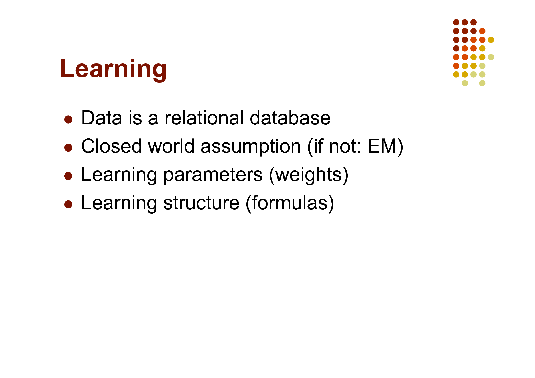
Learning
Data is a relational database Closed world assumption (if not: EM) Learning parameters (weights) Learning structure (formulas)
71
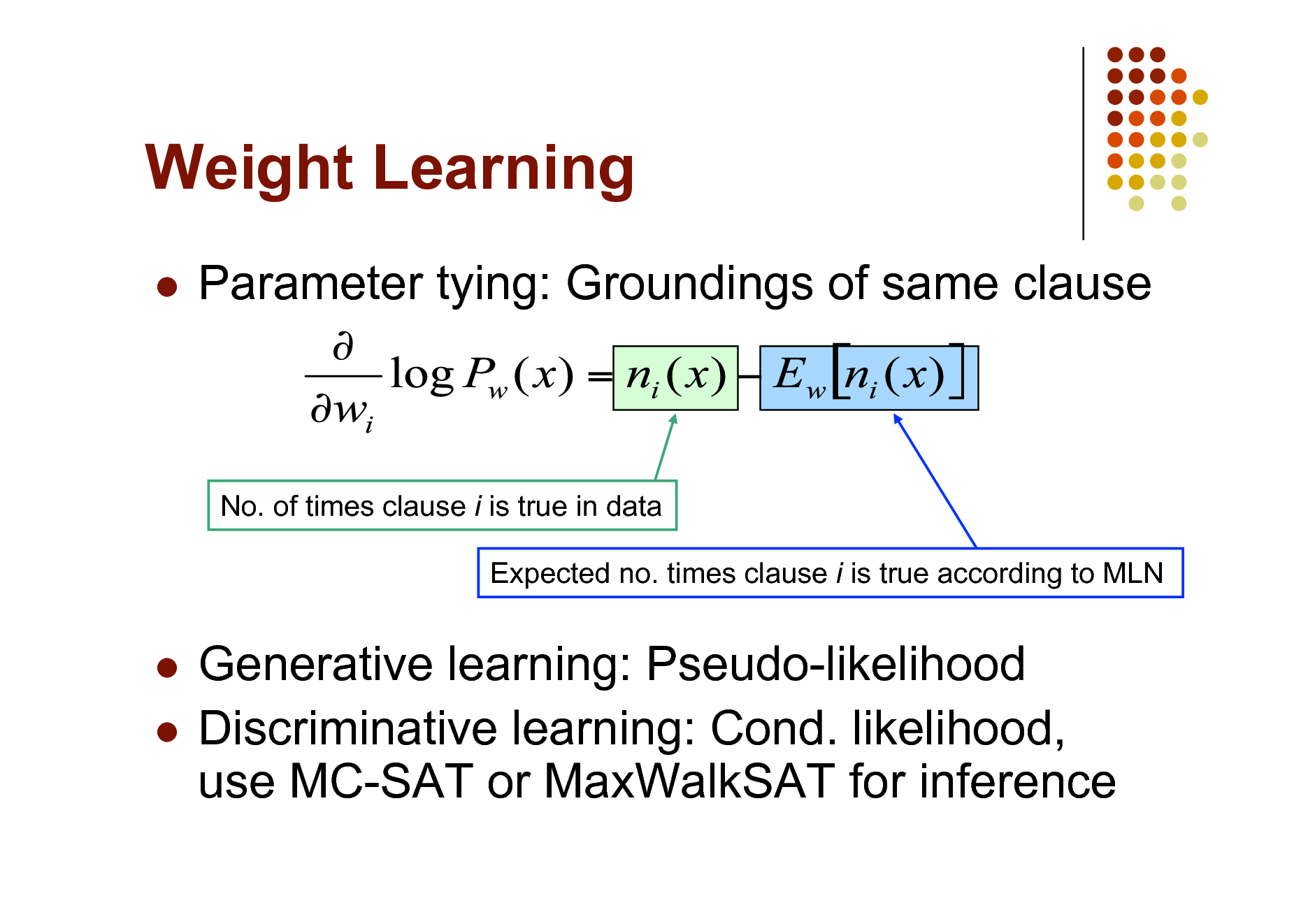
Weight Learning
Parameter tying: Groundings of same clause
No. of times clause i is true in data Expected no. times clause i is true according to MLN
Generative learning: Pseudo-likelihood Discriminative learning: Cond. likelihood, use MC-SAT or MaxWalkSAT for inference
72
Structure Learning
Generalizes feature induction in Markov nets Any inductive logic programming approach can be used, but . . . Goal is to induce any clauses, not just Horn Evaluation function should be likelihood Requires learning weights for each candidate Turns out not to be bottleneck Bottleneck is counting clause groundings Solution: Subsampling
73
![Slide: Structure Learning
Initial state: Unit clauses or hand-coded KB Operators: Add/remove literal, flip sign Evaluation function: Pseudo-likelihood + Structure prior Search: Beam, shortest-first, bottom-up
[Kok & Domingos, 2005; Mihalkova & Mooney, 2007]](https://yosinski.com/mlss12/media/slides/MLSS-2012-Domingos-Statistical-Relational-Learning_074.png)
Structure Learning
Initial state: Unit clauses or hand-coded KB Operators: Add/remove literal, flip sign Evaluation function: Pseudo-likelihood + Structure prior Search: Beam, shortest-first, bottom-up
[Kok & Domingos, 2005; Mihalkova & Mooney, 2007]
74
Alchemy
Open-source software including: Full first-order logic syntax Generative & discriminative weight learning Structure learning Weighted satisfiability and MCMC Programming language features alchemy.cs.washington.edu
75
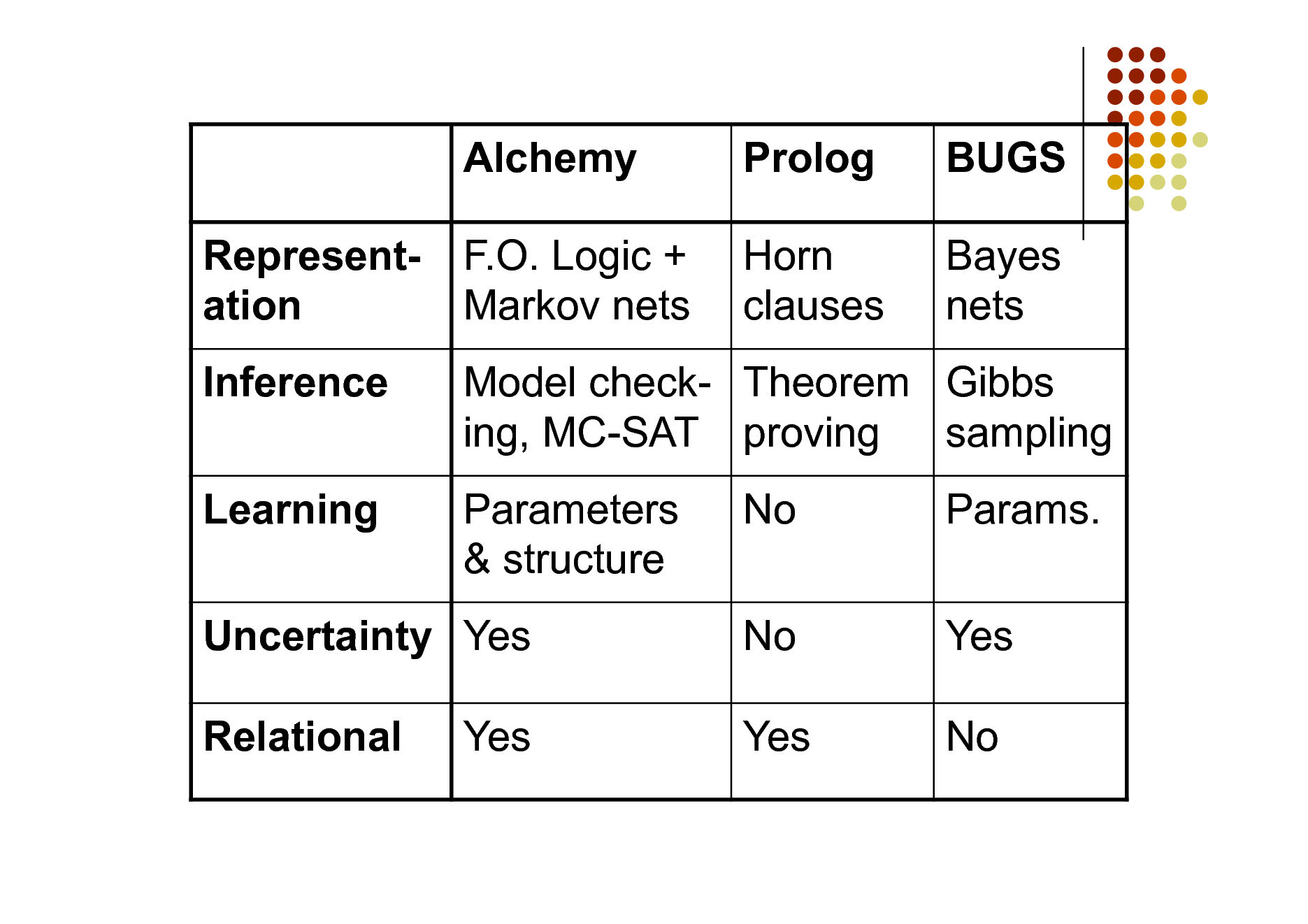
Alchemy Representation Inference Learning F.O. Logic + Markov nets
Prolog Horn clauses
BUGS Bayes nets
Model check- Theorem Gibbs ing, MC-SAT proving sampling Parameters & structure No No Yes Params. Yes No
Uncertainty Yes Relational Yes
76
Overview
Motivation Foundational areas
Probabilistic inference Statistical learning Logical inference Inductive logic programming
Putting the pieces together Applications
77
Applications
Basics Logistic regression Hypertext classification Information retrieval Entity resolution Hidden Markov models Information extraction
Statistical parsing Semantic processing Bayesian networks Relational models Robot mapping Planning and MDPs Practical tips
78
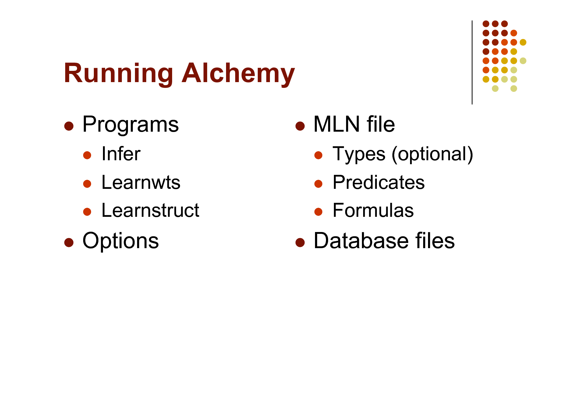
Running Alchemy
Programs
MLN file
Infer Learnwts Learnstruct
Types (optional) Predicates Formulas
Options
Database files
79
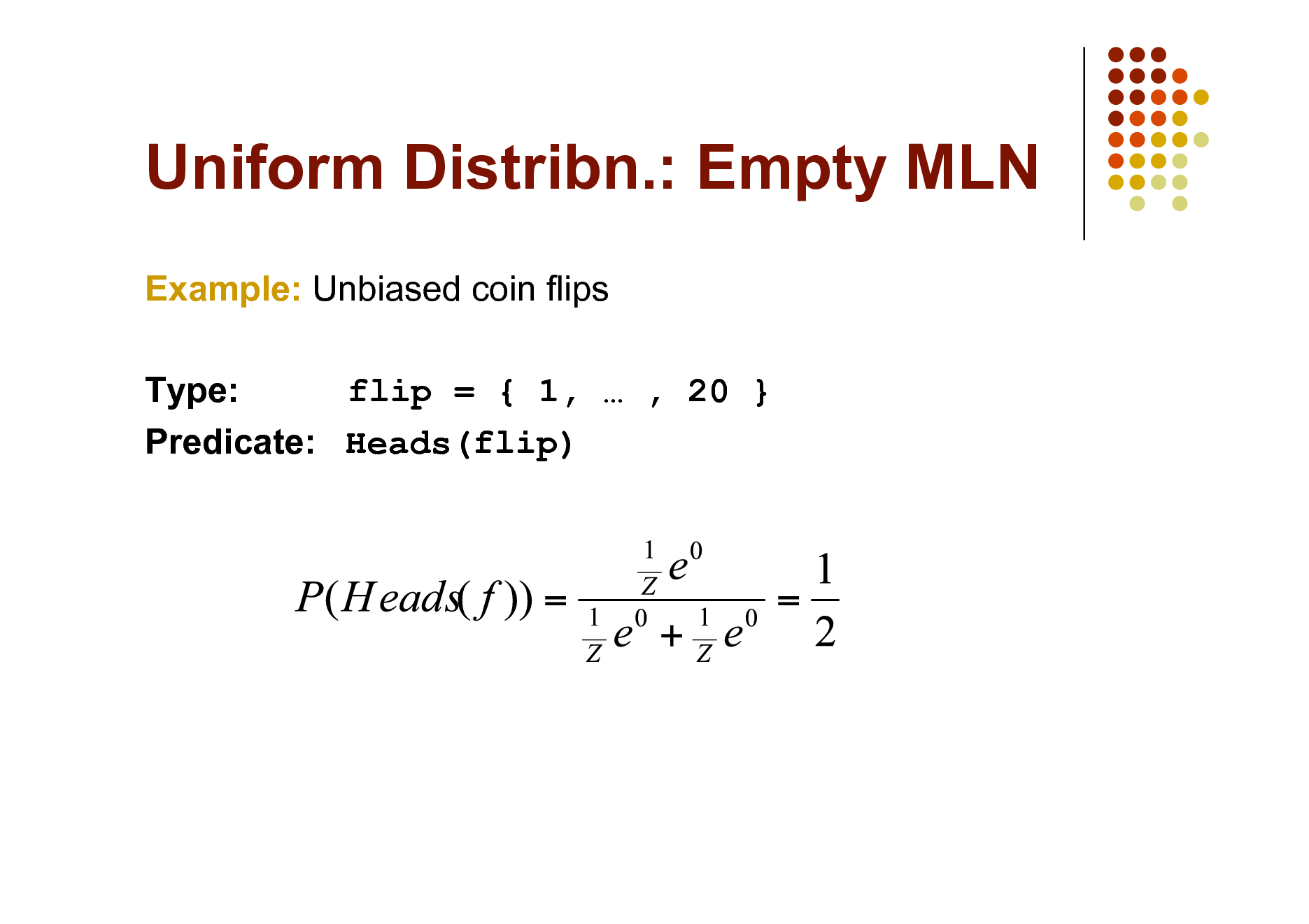
Uniform Distribn.: Empty MLN
Example: Unbiased coin flips Type: flip = { 1, , 20 } Predicate: Heads(flip)
80
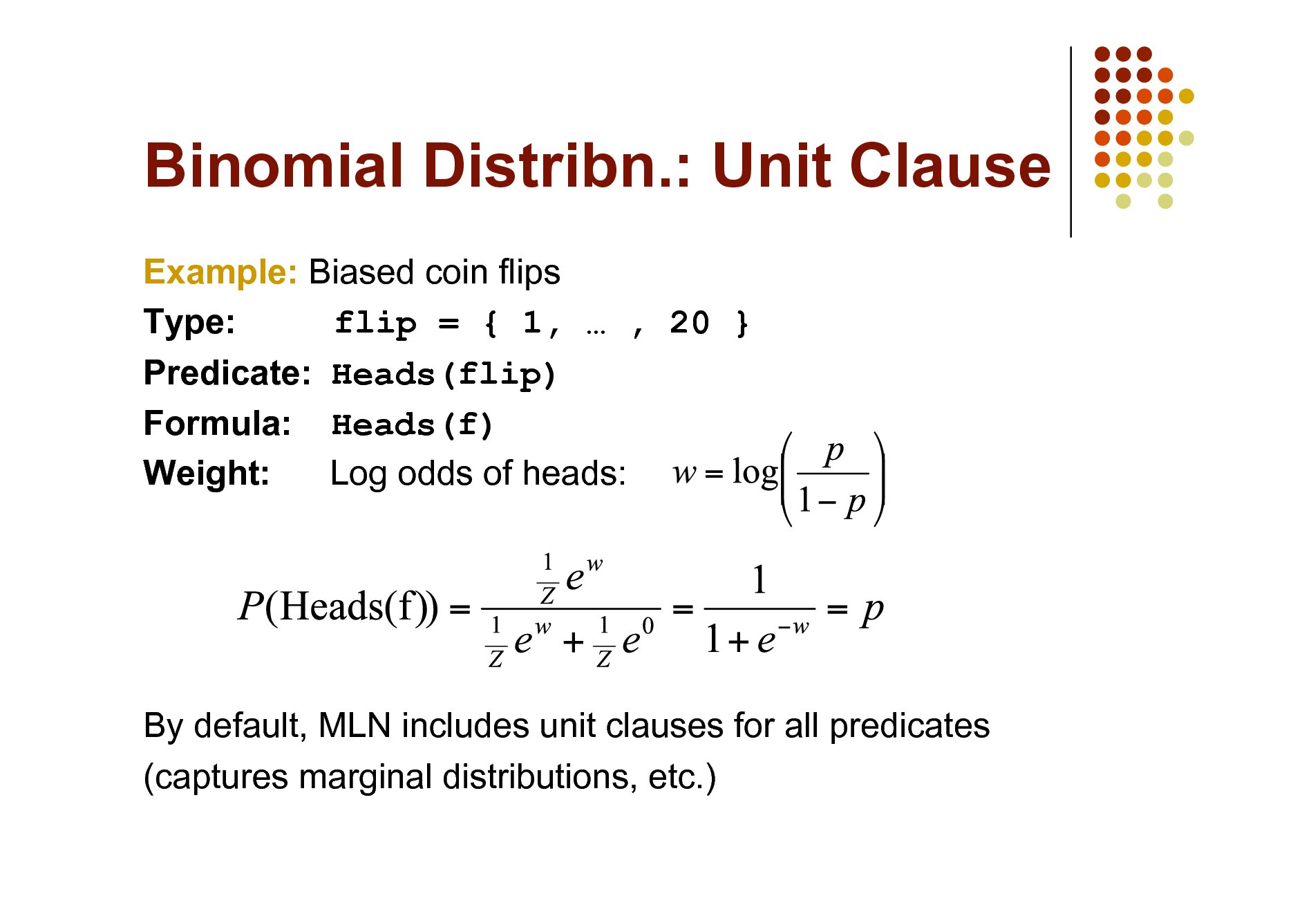
Binomial Distribn.: Unit Clause
Example: Biased coin flips Type: flip = { 1, , 20 } Predicate: Heads(flip) Formula: Heads(f) Weight: Log odds of heads:
By default, MLN includes unit clauses for all predicates (captures marginal distributions, etc.)
81
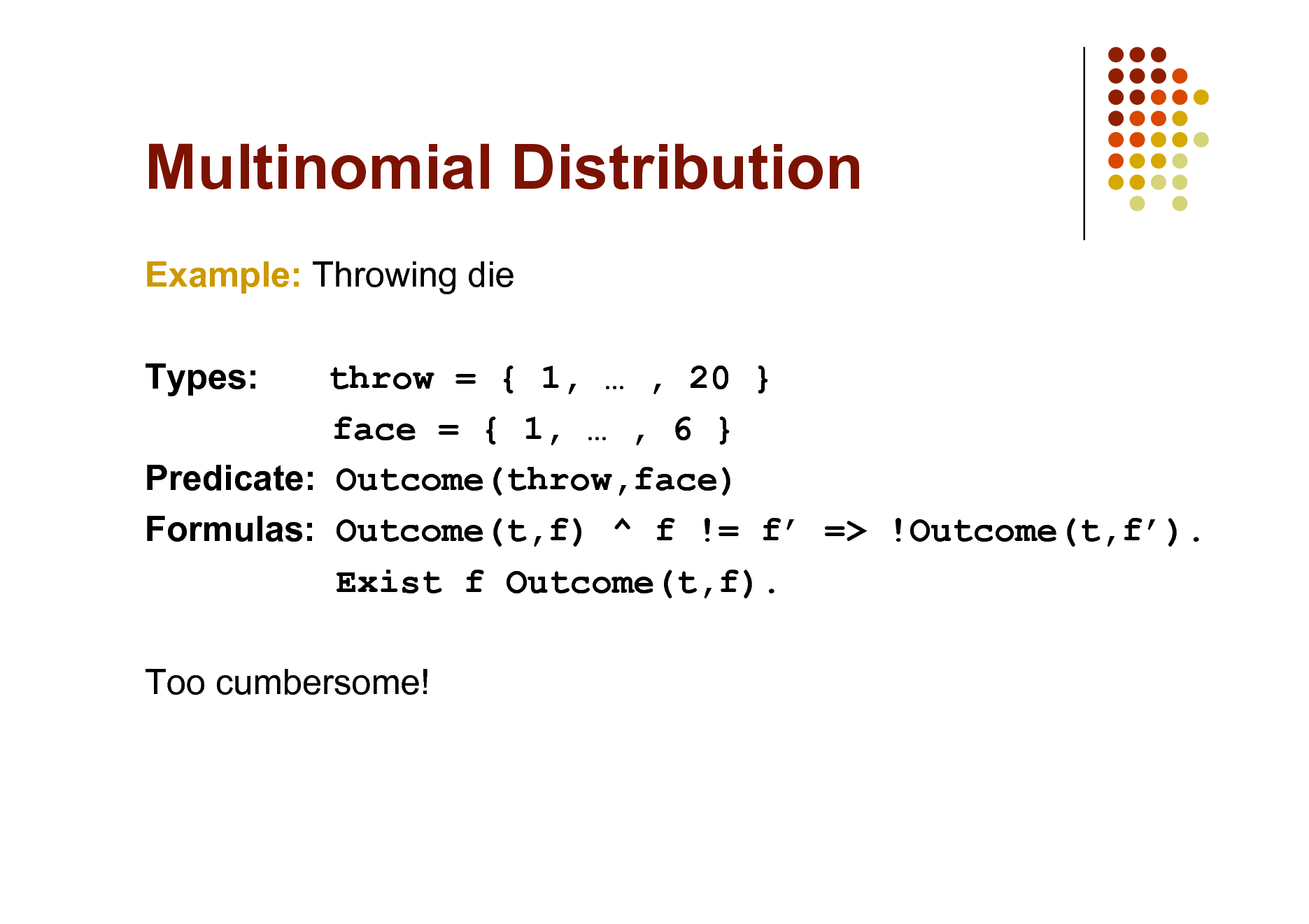
Multinomial Distribution
Example: Throwing die Types: throw = { 1, , 20 } face = { 1, , 6 } Predicate: Outcome(throw,face) Formulas: Outcome(t,f) ^ f != f => !Outcome(t,f). Exist f Outcome(t,f). Too cumbersome!
82
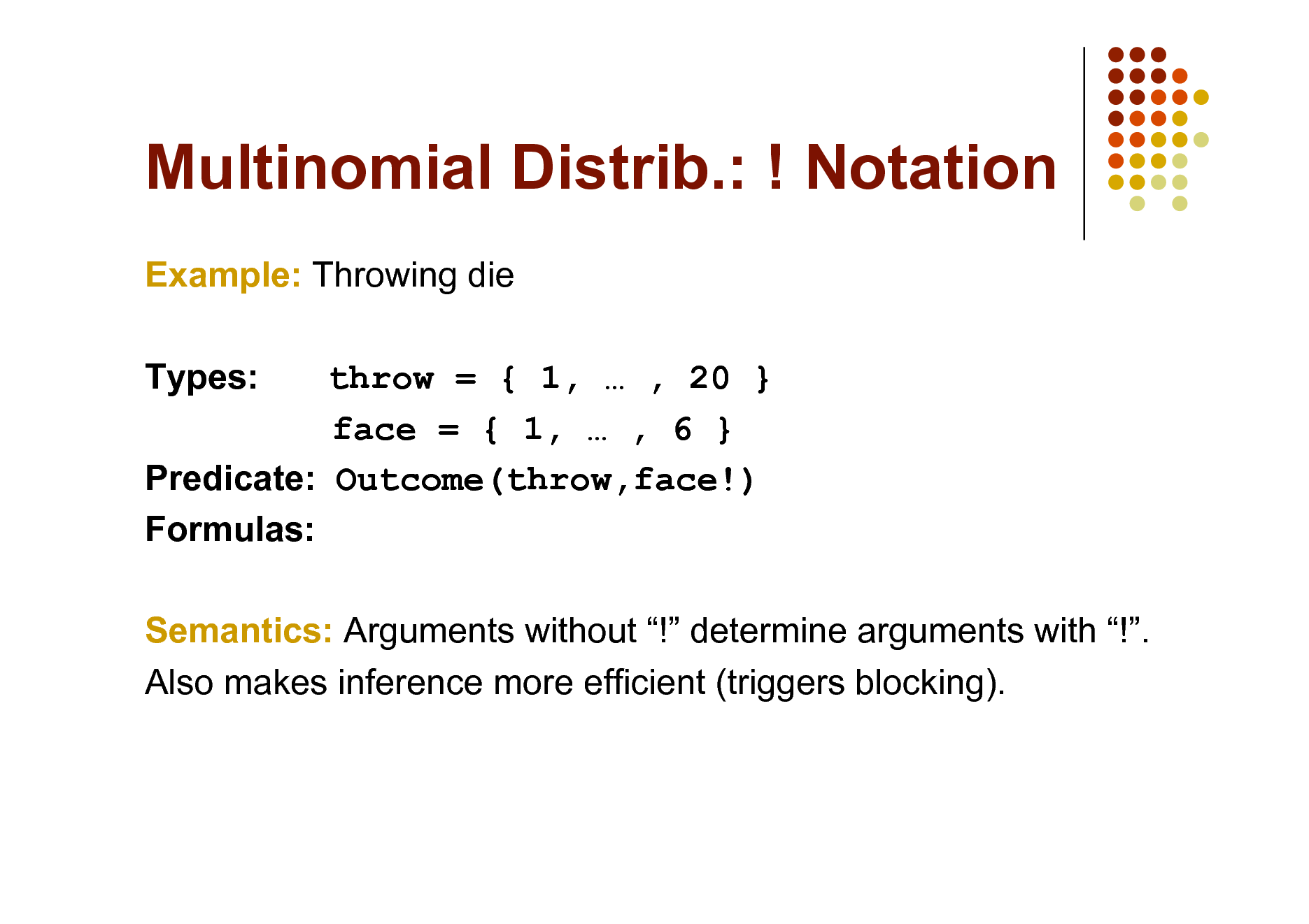
Multinomial Distrib.: ! Notation
Example: Throwing die Types: throw = { 1, , 20 } face = { 1, , 6 } Predicate: Outcome(throw,face!) Formulas: Semantics: Arguments without ! determine arguments with !. Also makes inference more efficient (triggers blocking).
83
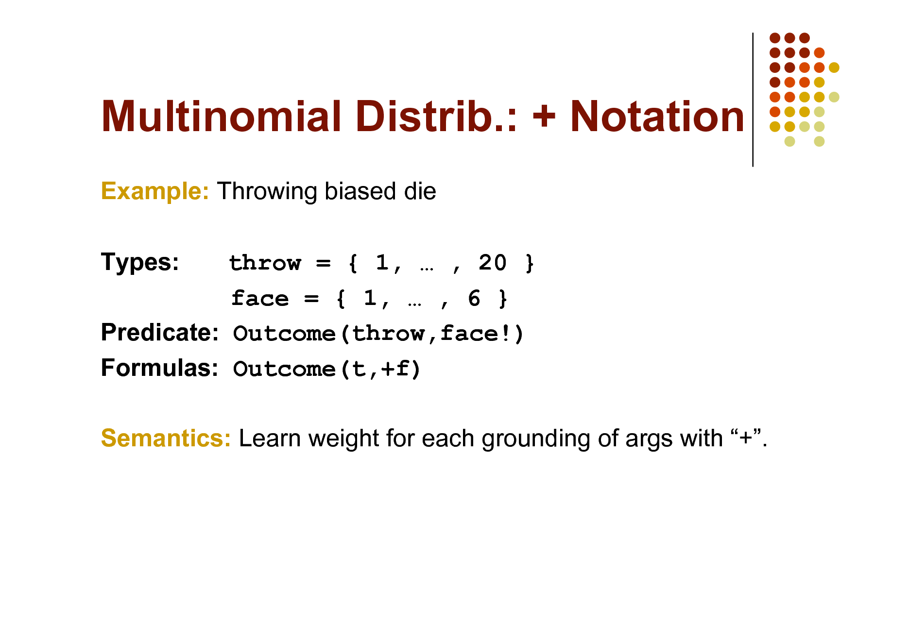
Multinomial Distrib.: + Notation
Example: Throwing biased die Types: throw = { 1, , 20 } face = { 1, , 6 } Predicate: Outcome(throw,face!) Formulas: Outcome(t,+f) Semantics: Learn weight for each grounding of args with +.
84
Logistic Regression
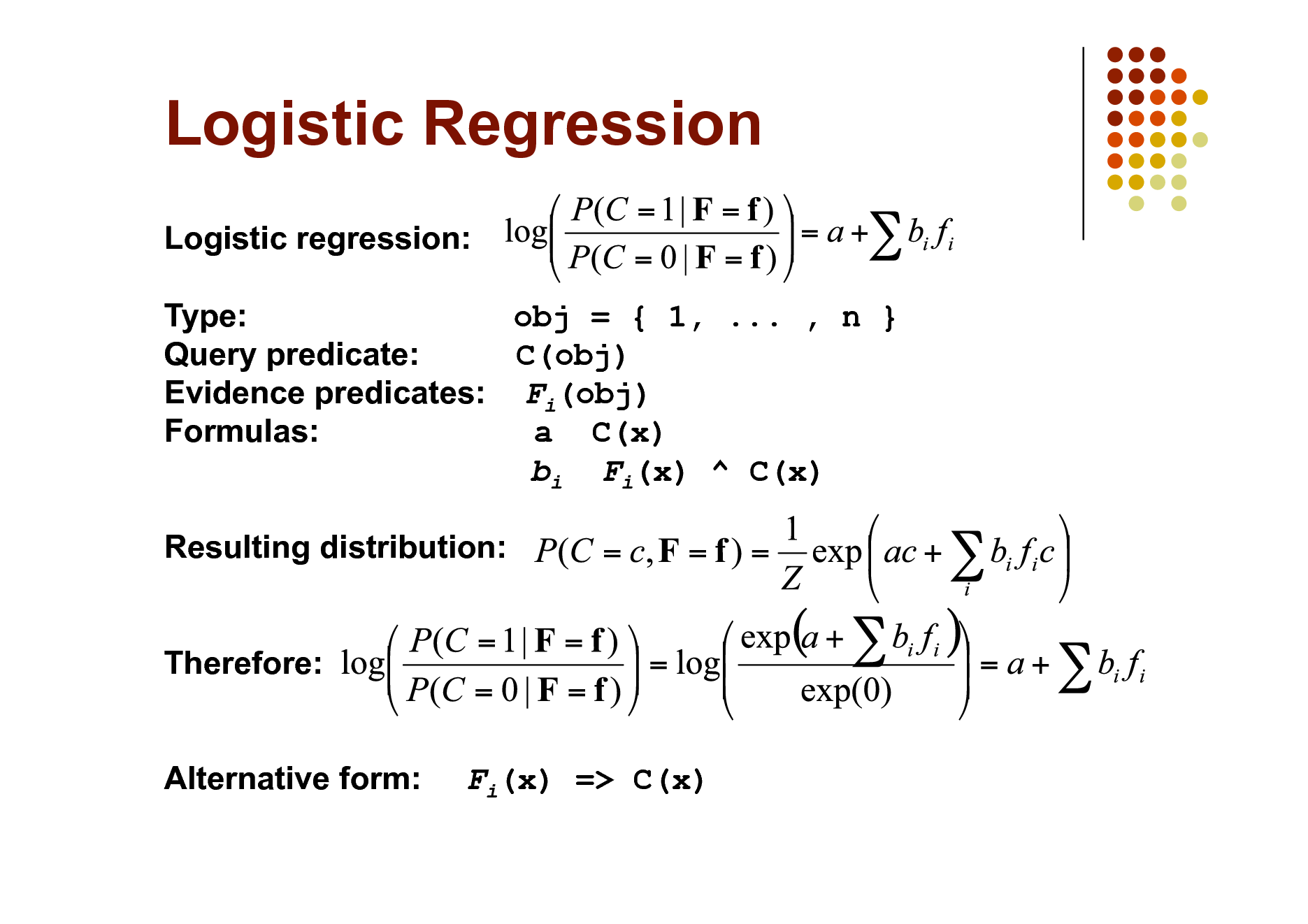
Logistic regression: Type: obj = { 1, ... , n } Query predicate: C(obj) Evidence predicates: Fi(obj) Formulas: a C(x) bi Fi(x) ^ C(x) Resulting distribution: Therefore: Alternative form:
Fi(x) => C(x)
85
Text Classification
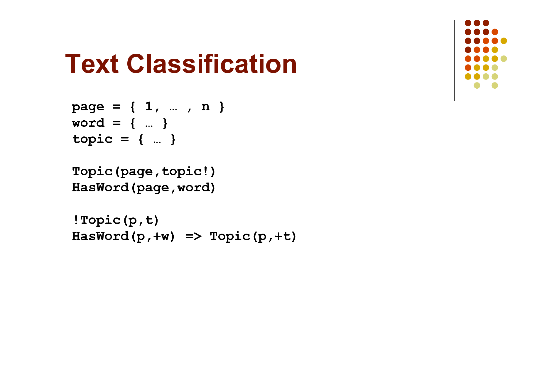
page = { 1, , n } word = { } topic = { } Topic(page,topic!) HasWord(page,word) !Topic(p,t) HasWord(p,+w) => Topic(p,+t)
86
Text Classification
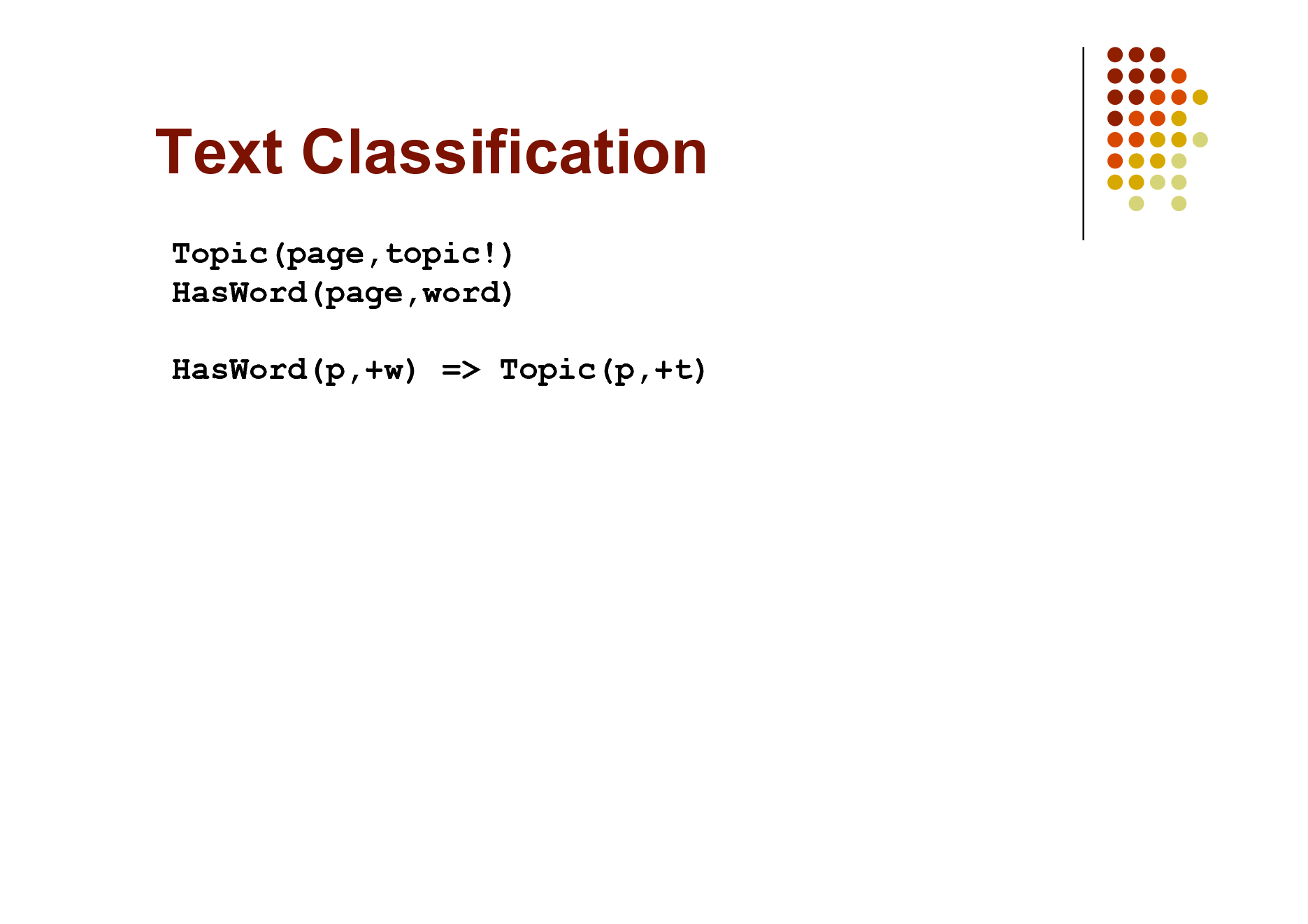
Topic(page,topic!) HasWord(page,word) HasWord(p,+w) => Topic(p,+t)
87
Hypertext Classification
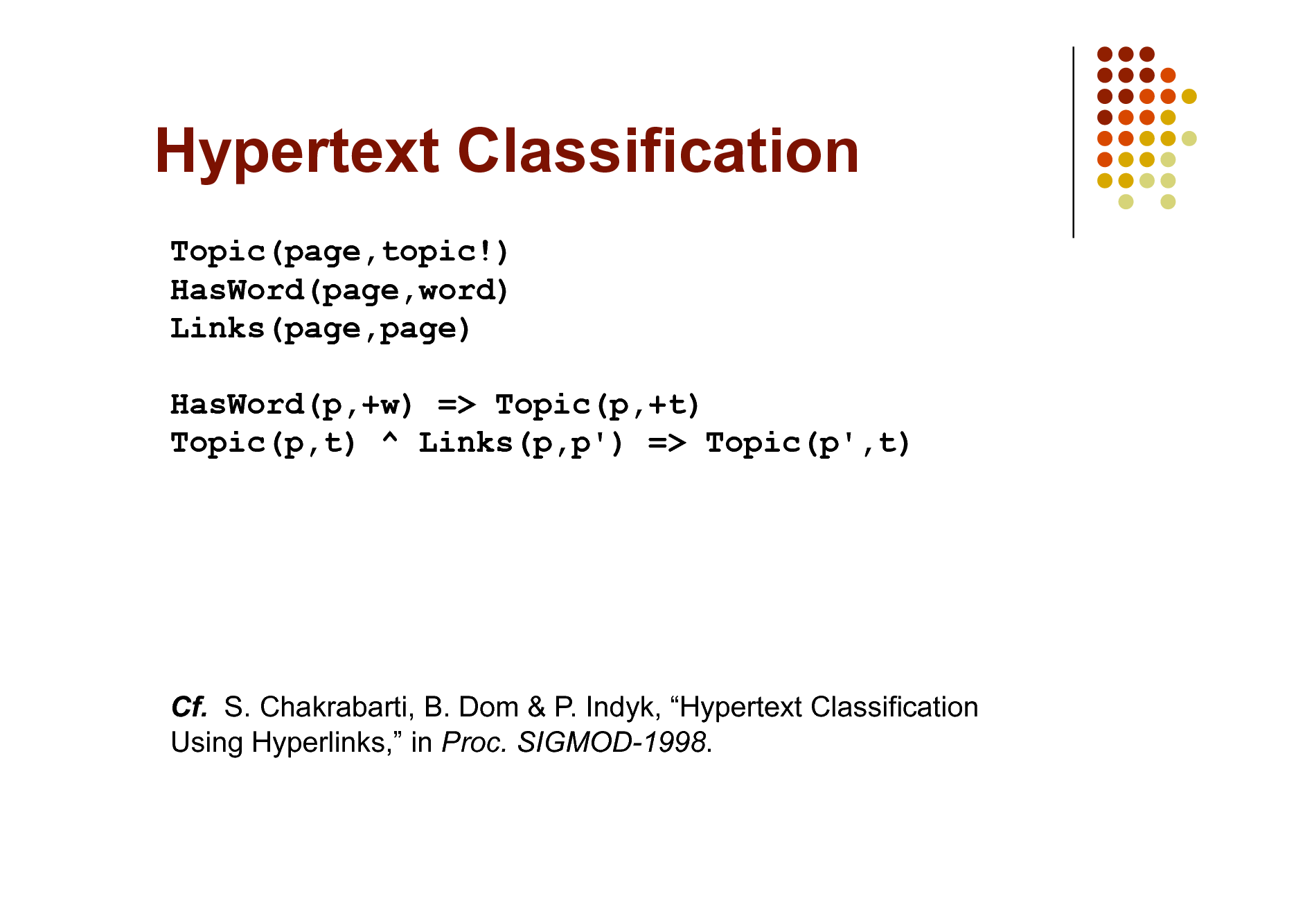
Topic(page,topic!) HasWord(page,word) Links(page,page) HasWord(p,+w) => Topic(p,+t) Topic(p,t) ^ Links(p,p') => Topic(p',t)
Cf. S. Chakrabarti, B. Dom & P. Indyk, Hypertext Classification Using Hyperlinks, in Proc. SIGMOD-1998.
88
Information Retrieval
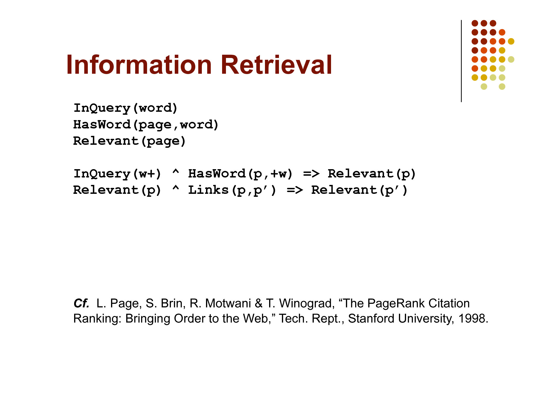
InQuery(word) HasWord(page,word) Relevant(page) InQuery(w+) ^ HasWord(p,+w) => Relevant(p) Relevant(p) ^ Links(p,p) => Relevant(p)
Cf. L. Page, S. Brin, R. Motwani & T. Winograd, The PageRank Citation Ranking: Bringing Order to the Web, Tech. Rept., Stanford University, 1998.
89
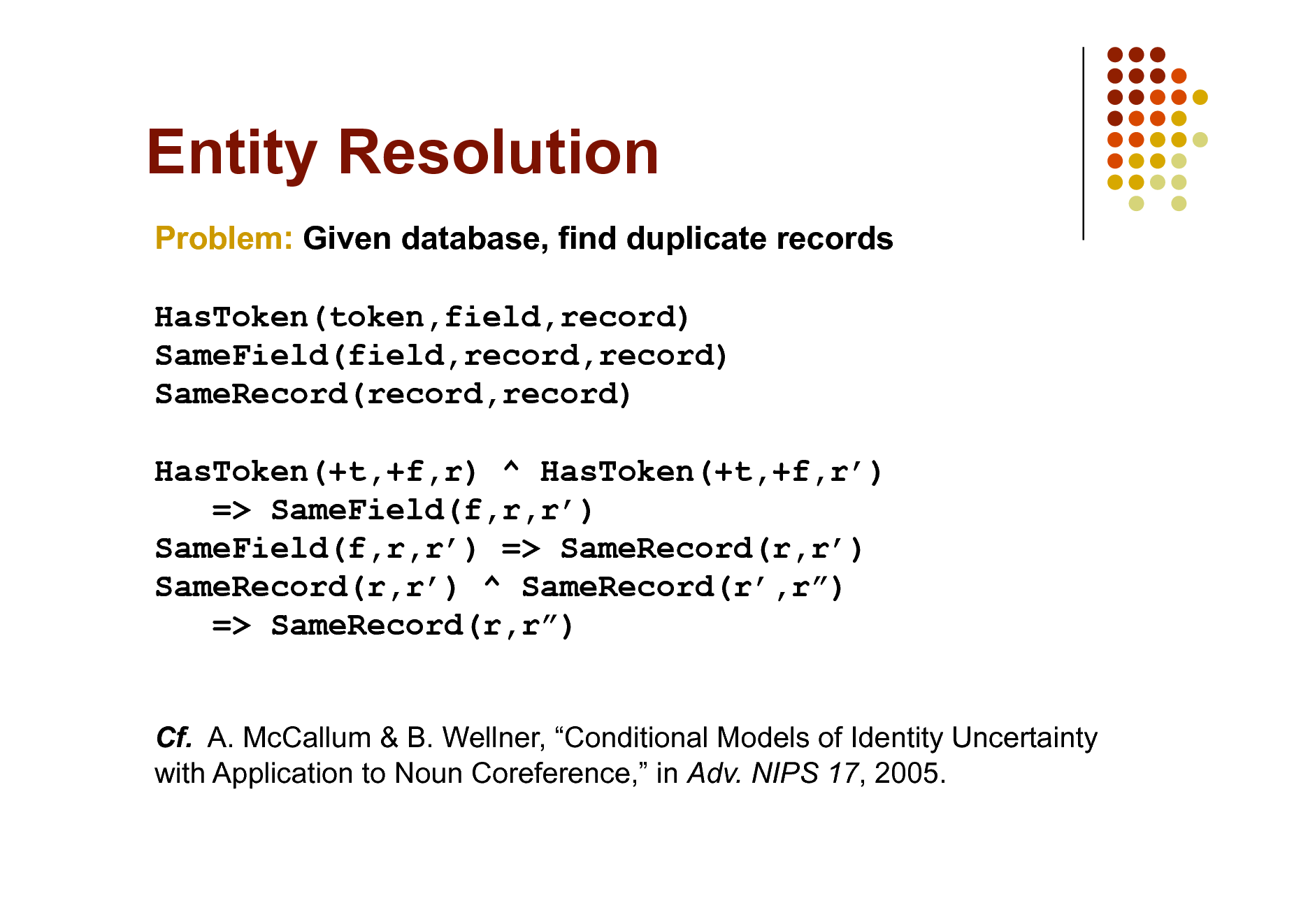
Entity Resolution
Problem: Given database, find duplicate records HasToken(token,field,record) SameField(field,record,record) SameRecord(record,record) HasToken(+t,+f,r) ^ HasToken(+t,+f,r) => SameField(f,r,r) SameField(f,r,r) => SameRecord(r,r) SameRecord(r,r) ^ SameRecord(r,r) => SameRecord(r,r)
Cf. A. McCallum & B. Wellner, Conditional Models of Identity Uncertainty with Application to Noun Coreference, in Adv. NIPS 17, 2005.
90
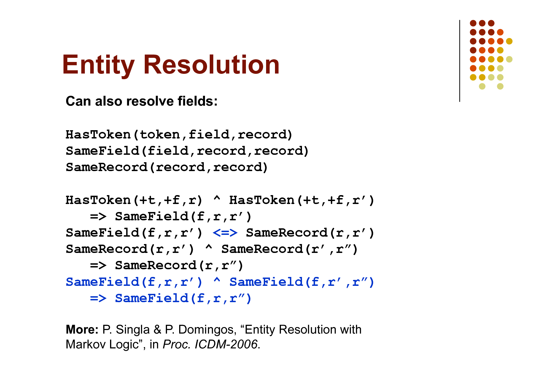
Entity Resolution
Can also resolve fields: HasToken(token,field,record) SameField(field,record,record) SameRecord(record,record) HasToken(+t,+f,r) ^ HasToken(+t,+f,r) => SameField(f,r,r) SameField(f,r,r) <=> SameRecord(r,r) SameRecord(r,r) ^ SameRecord(r,r) => SameRecord(r,r) SameField(f,r,r) ^ SameField(f,r,r) => SameField(f,r,r)
More: P. Singla & P. Domingos, Entity Resolution with Markov Logic, in Proc. ICDM-2006.
91
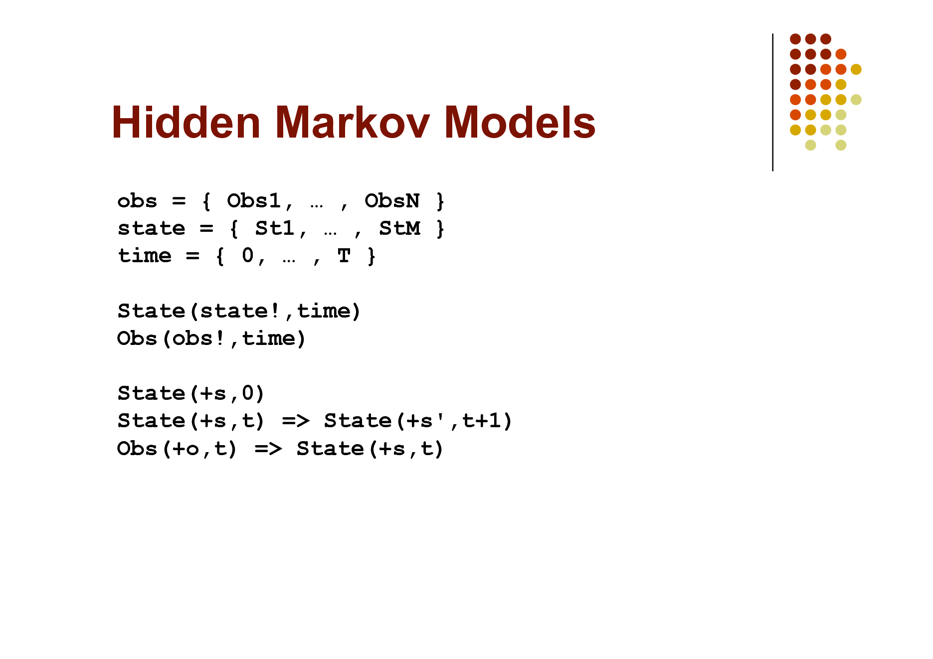
Hidden Markov Models
obs = { Obs1, , ObsN } state = { St1, , StM } time = { 0, , T } State(state!,time) Obs(obs!,time) State(+s,0) State(+s,t) => State(+s',t+1) Obs(+o,t) => State(+s,t)
92
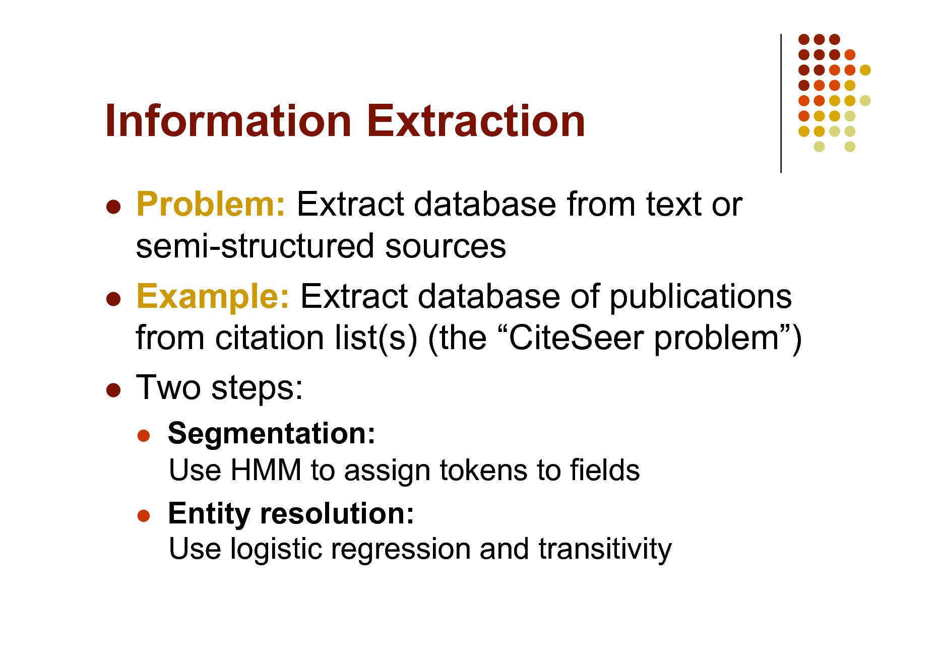
Information Extraction
Problem: Extract database from text or semi-structured sources Example: Extract database of publications from citation list(s) (the CiteSeer problem) Two steps:
Segmentation: Use HMM to assign tokens to fields Entity resolution: Use logistic regression and transitivity
93
Information Extraction
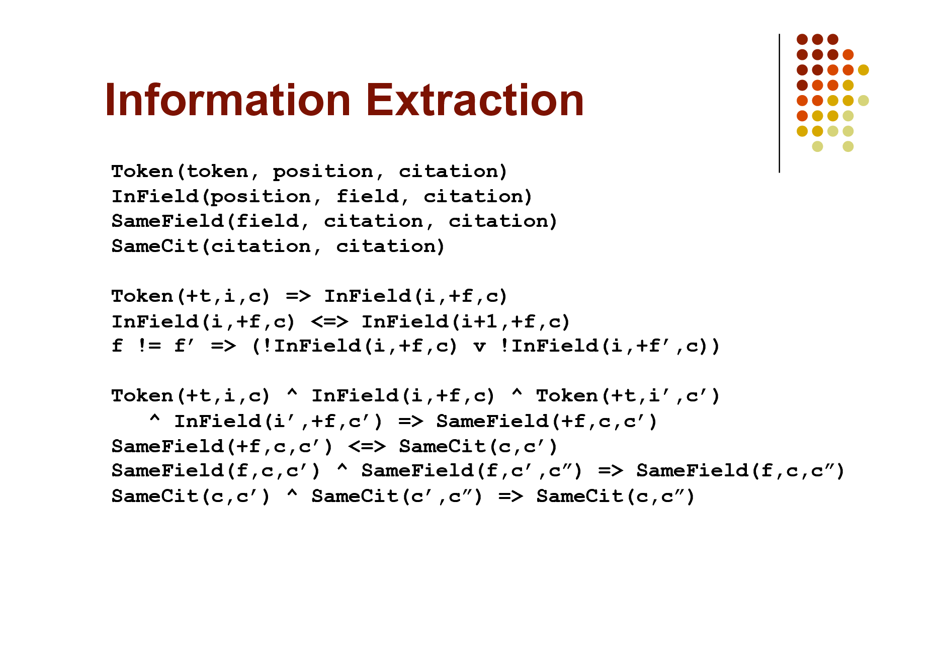
Token(token, position, citation) InField(position, field, citation) SameField(field, citation, citation) SameCit(citation, citation) Token(+t,i,c) => InField(i,+f,c) InField(i,+f,c) <=> InField(i+1,+f,c) f != f => (!InField(i,+f,c) v !InField(i,+f,c)) Token(+t,i,c) ^ InField(i,+f,c) ^ Token(+t,i,c) ^ InField(i,+f,c) => SameField(+f,c,c) SameField(+f,c,c) <=> SameCit(c,c) SameField(f,c,c) ^ SameField(f,c,c) => SameField(f,c,c) SameCit(c,c) ^ SameCit(c,c) => SameCit(c,c)
94
Information Extraction
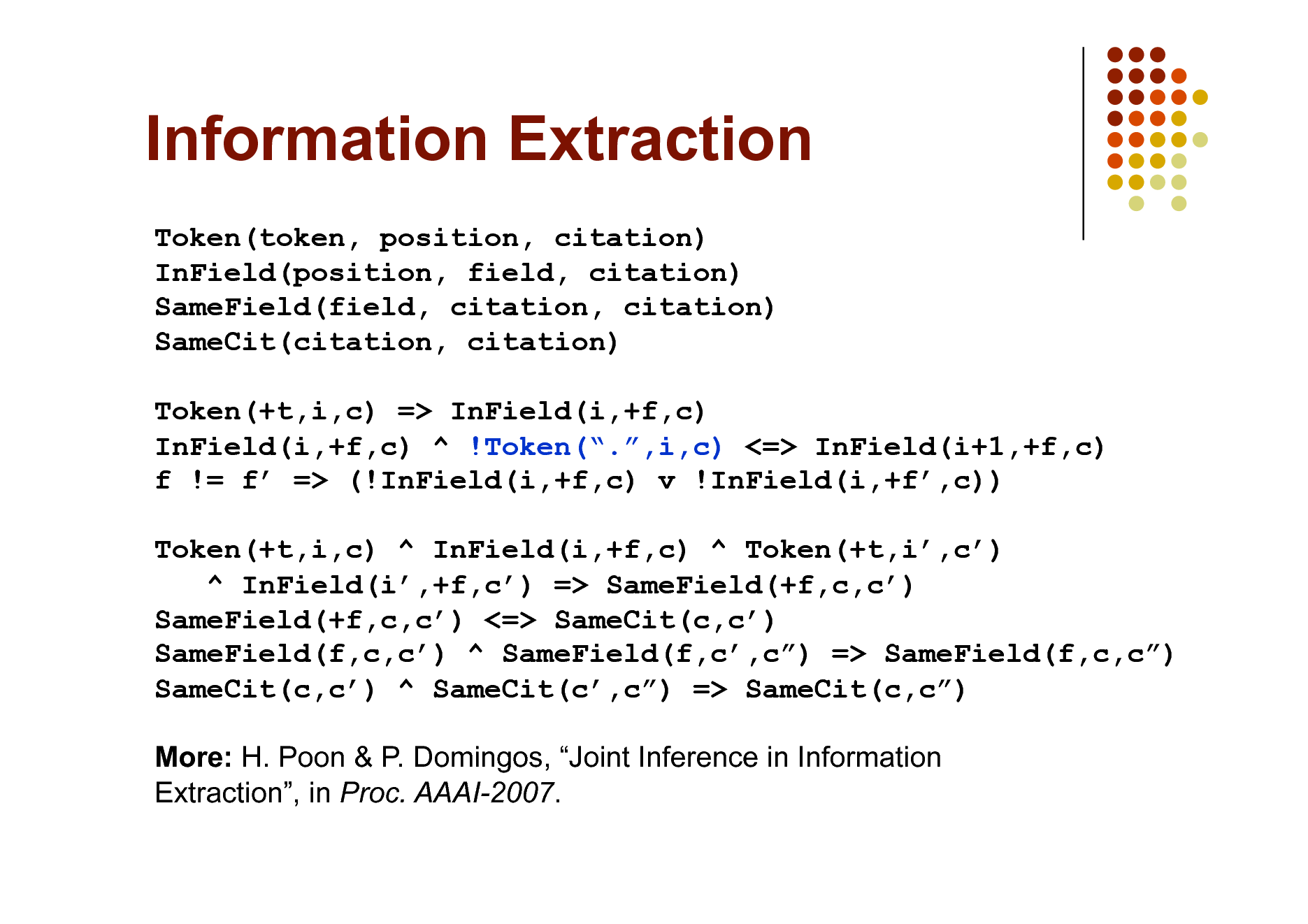
Token(token, position, citation) InField(position, field, citation) SameField(field, citation, citation) SameCit(citation, citation) Token(+t,i,c) => InField(i,+f,c) InField(i,+f,c) ^ !Token(.,i,c) <=> InField(i+1,+f,c) f != f => (!InField(i,+f,c) v !InField(i,+f,c)) Token(+t,i,c) ^ InField(i,+f,c) ^ Token(+t,i,c) ^ InField(i,+f,c) => SameField(+f,c,c) SameField(+f,c,c) <=> SameCit(c,c) SameField(f,c,c) ^ SameField(f,c,c) => SameField(f,c,c) SameCit(c,c) ^ SameCit(c,c) => SameCit(c,c) More: H. Poon & P. Domingos, Joint Inference in Information Extraction, in Proc. AAAI-2007.
95
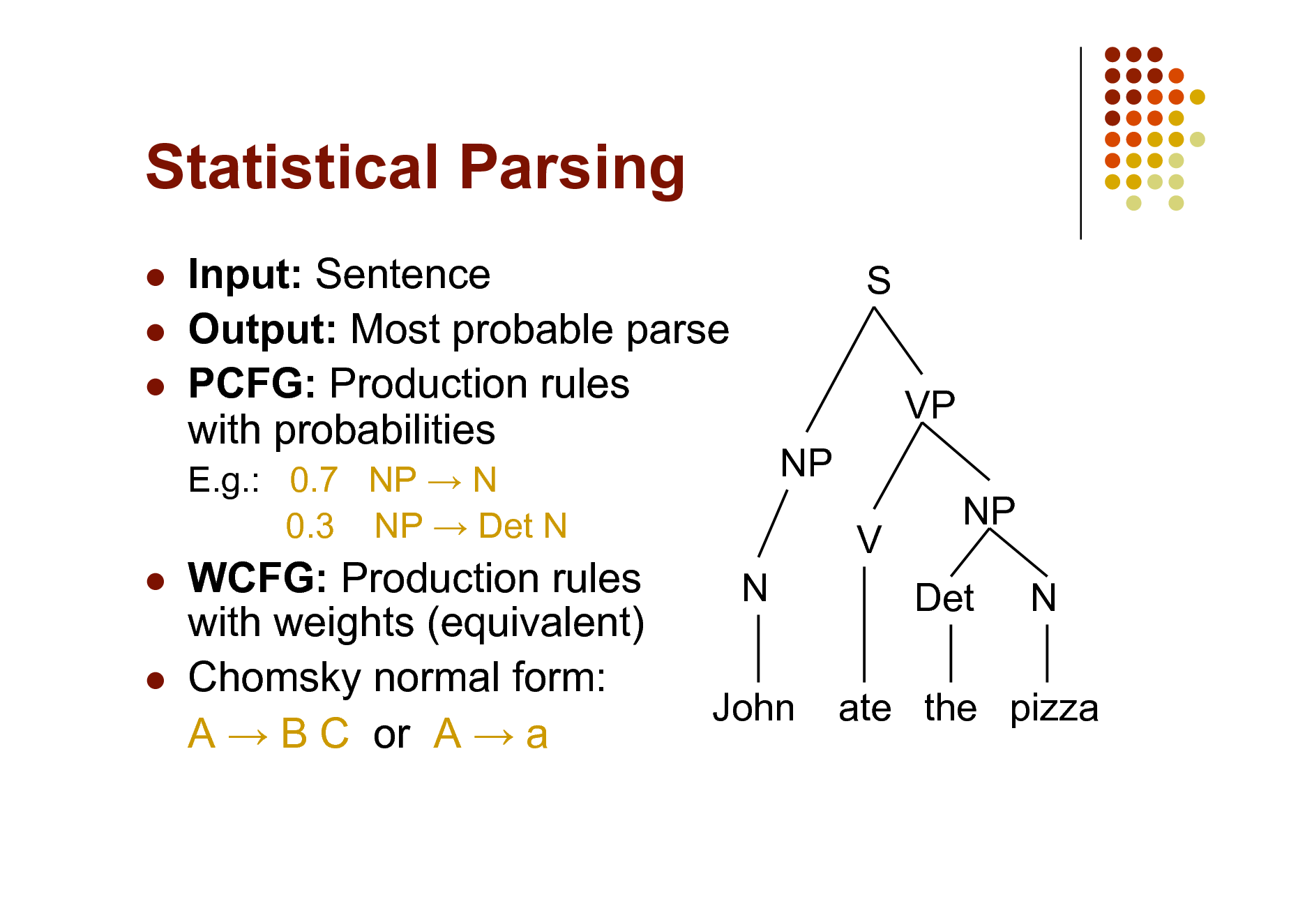
Statistical Parsing
Input: Sentence Output: Most probable parse PCFG: Production rules with probabilities
E.g.: 0.7 NP N 0.3 NP Det N
S VP NP V N NP Det N
WCFG: Production rules with weights (equivalent) Chomsky normal form: A B C or A a
John
ate the pizza
96
Statistical Parsing
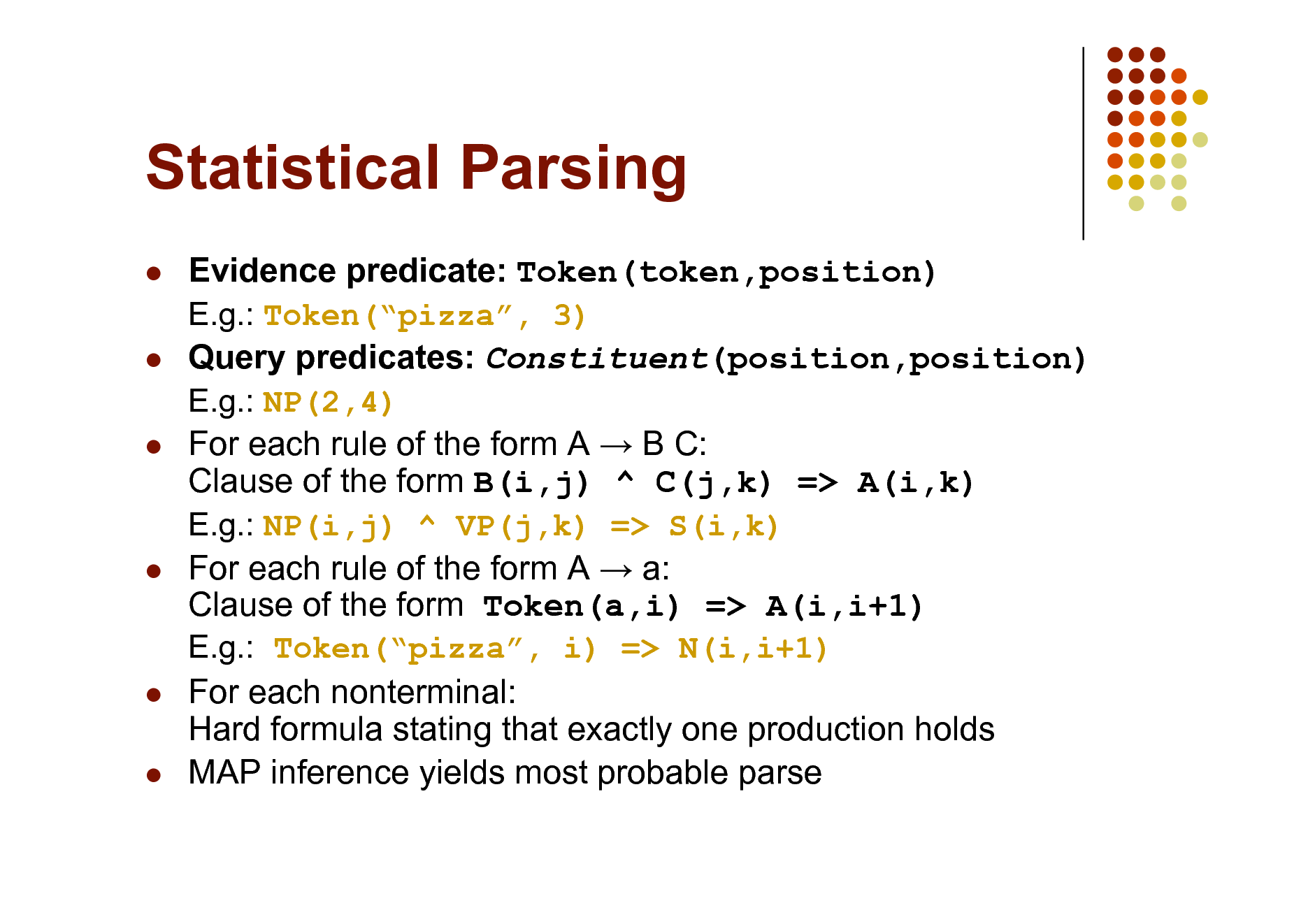
Evidence predicate: Token(token,position) E.g.: Token(pizza, 3) Query predicates: Constituent(position,position) E.g.: NP(2,4) For each rule of the form A B C: Clause of the form B(i,j) ^ C(j,k) => A(i,k) E.g.: NP(i,j) ^ VP(j,k) => S(i,k) For each rule of the form A a: Clause of the form Token(a,i) => A(i,i+1) E.g.: Token(pizza, i) => N(i,i+1) For each nonterminal: Hard formula stating that exactly one production holds MAP inference yields most probable parse
97
Semantic Processing
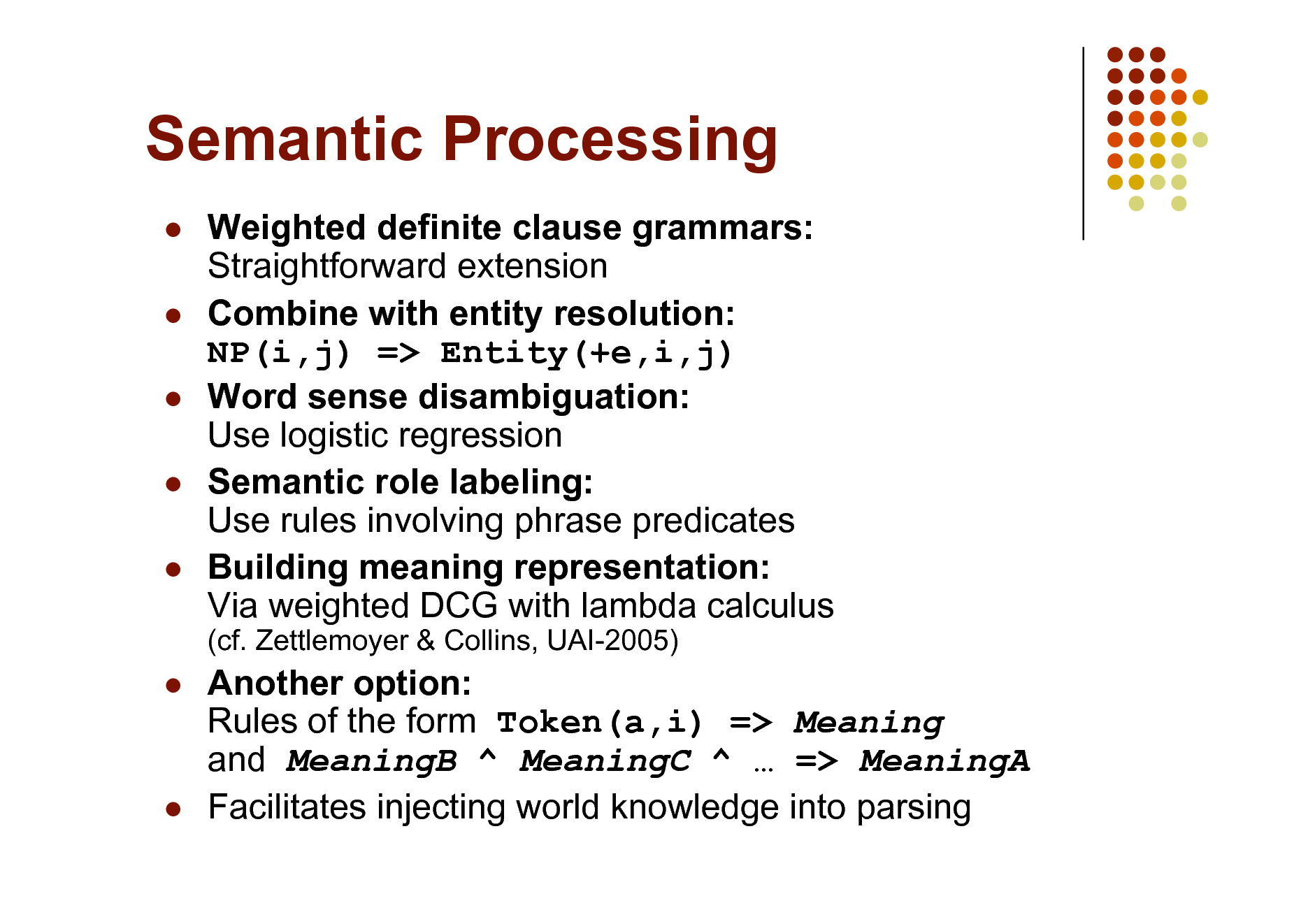
Weighted definite clause grammars: Straightforward extension Combine with entity resolution: NP(i,j) => Entity(+e,i,j) Word sense disambiguation: Use logistic regression Semantic role labeling: Use rules involving phrase predicates Building meaning representation: Via weighted DCG with lambda calculus
(cf. Zettlemoyer & Collins, UAI-2005)
Another option: Rules of the form Token(a,i) => Meaning and MeaningB ^ MeaningC ^ => MeaningA Facilitates injecting world knowledge into parsing
98
Semantic Processing
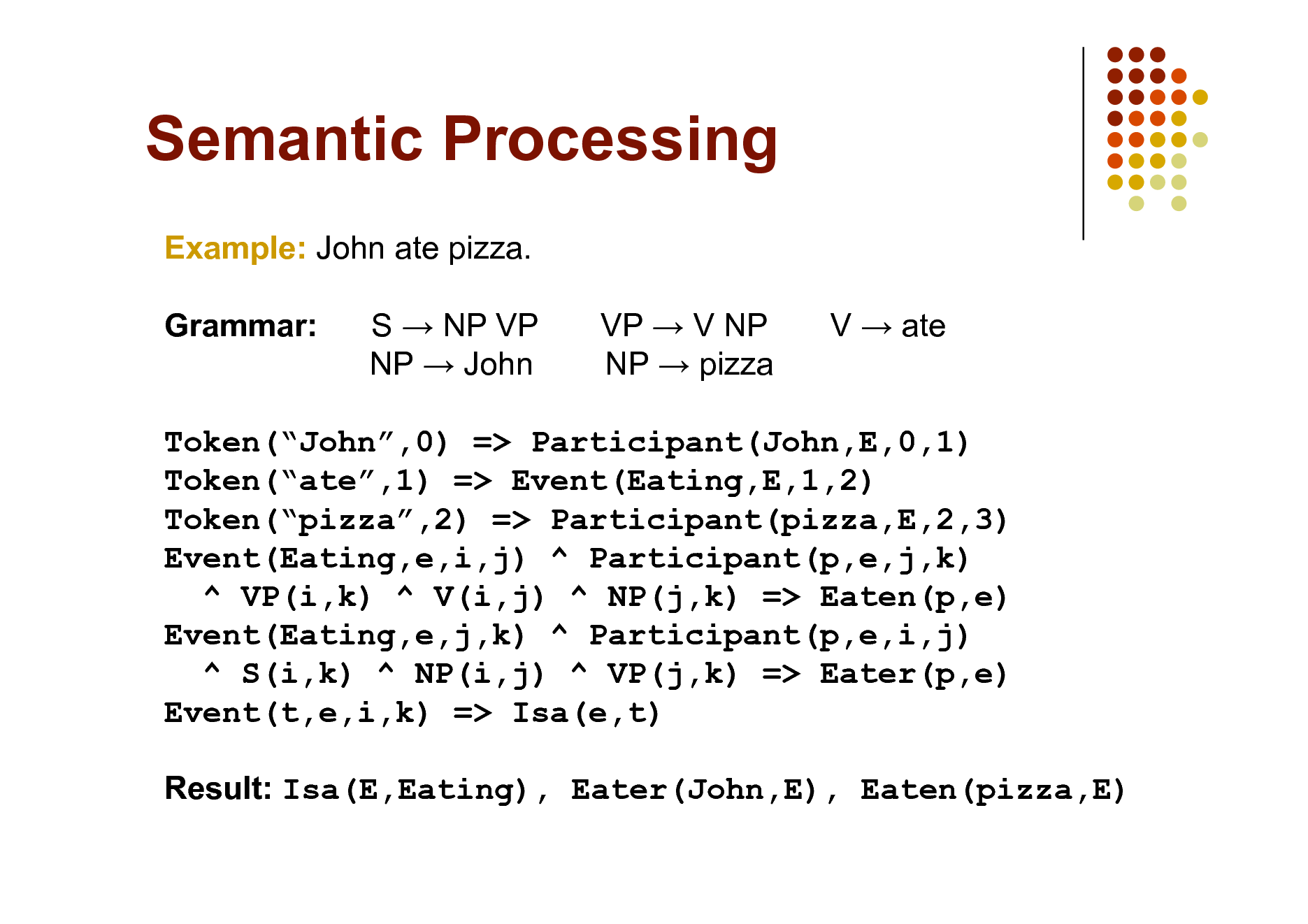
Example: John ate pizza. Grammar: S NP VP NP John VP V NP NP pizza V ate
Token(John,0) => Participant(John,E,0,1) Token(ate,1) => Event(Eating,E,1,2) Token(pizza,2) => Participant(pizza,E,2,3) Event(Eating,e,i,j) ^ Participant(p,e,j,k) ^ VP(i,k) ^ V(i,j) ^ NP(j,k) => Eaten(p,e) Event(Eating,e,j,k) ^ Participant(p,e,i,j) ^ S(i,k) ^ NP(i,j) ^ VP(j,k) => Eater(p,e) Event(t,e,i,k) => Isa(e,t) Result: Isa(E,Eating), Eater(John,E), Eaten(pizza,E)
99
Bayesian Networks
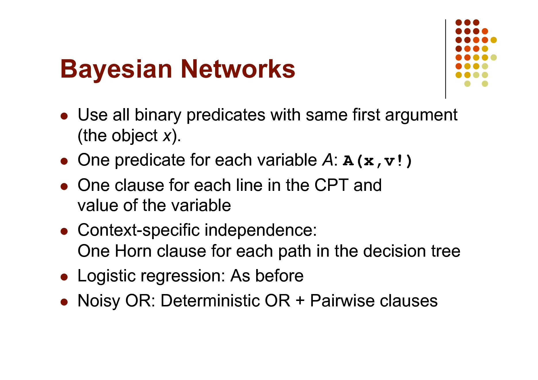
Use all binary predicates with same first argument (the object x). One predicate for each variable A: A(x,v!) One clause for each line in the CPT and value of the variable Context-specific independence: One Horn clause for each path in the decision tree Logistic regression: As before Noisy OR: Deterministic OR + Pairwise clauses
100
Relational Models
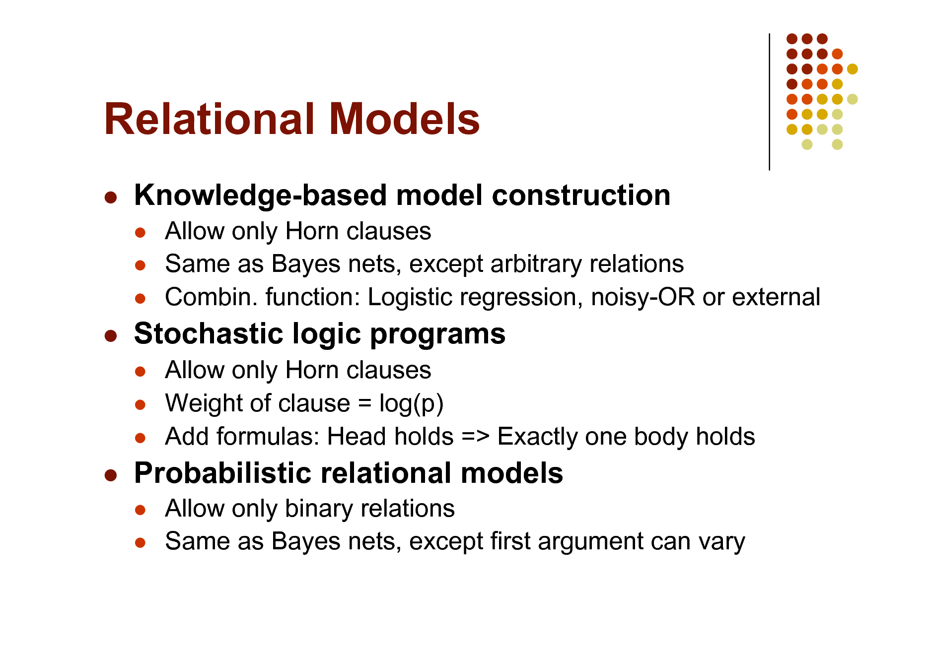
Knowledge-based model construction
Allow only Horn clauses Same as Bayes nets, except arbitrary relations Combin. function: Logistic regression, noisy-OR or external Allow only Horn clauses Weight of clause = log(p) Add formulas: Head holds => Exactly one body holds Allow only binary relations Same as Bayes nets, except first argument can vary
Stochastic logic programs
Probabilistic relational models
101
Relational Models
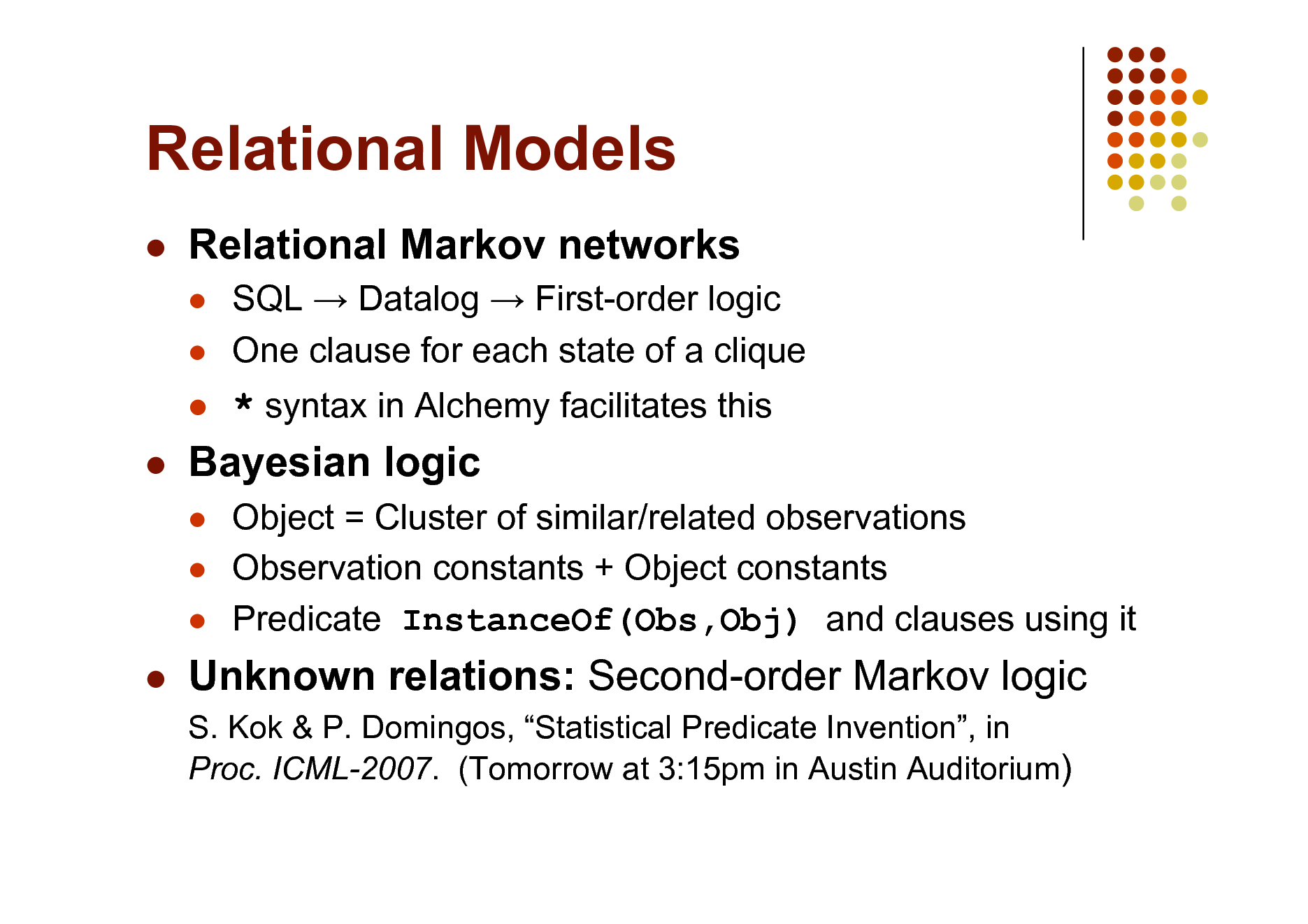
Relational Markov networks
SQL Datalog First-order logic One clause for each state of a clique
* syntax in Alchemy facilitates this
Object = Cluster of similar/related observations Observation constants + Object constants Predicate InstanceOf(Obs,Obj) and clauses using it
Bayesian logic
Unknown relations: Second-order Markov logic
S. Kok & P. Domingos, Statistical Predicate Invention, in Proc. ICML-2007. (Tomorrow at 3:15pm in Austin Auditorium)
102
Robot Mapping
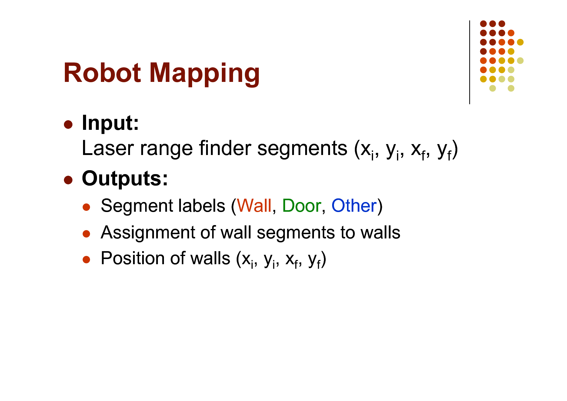
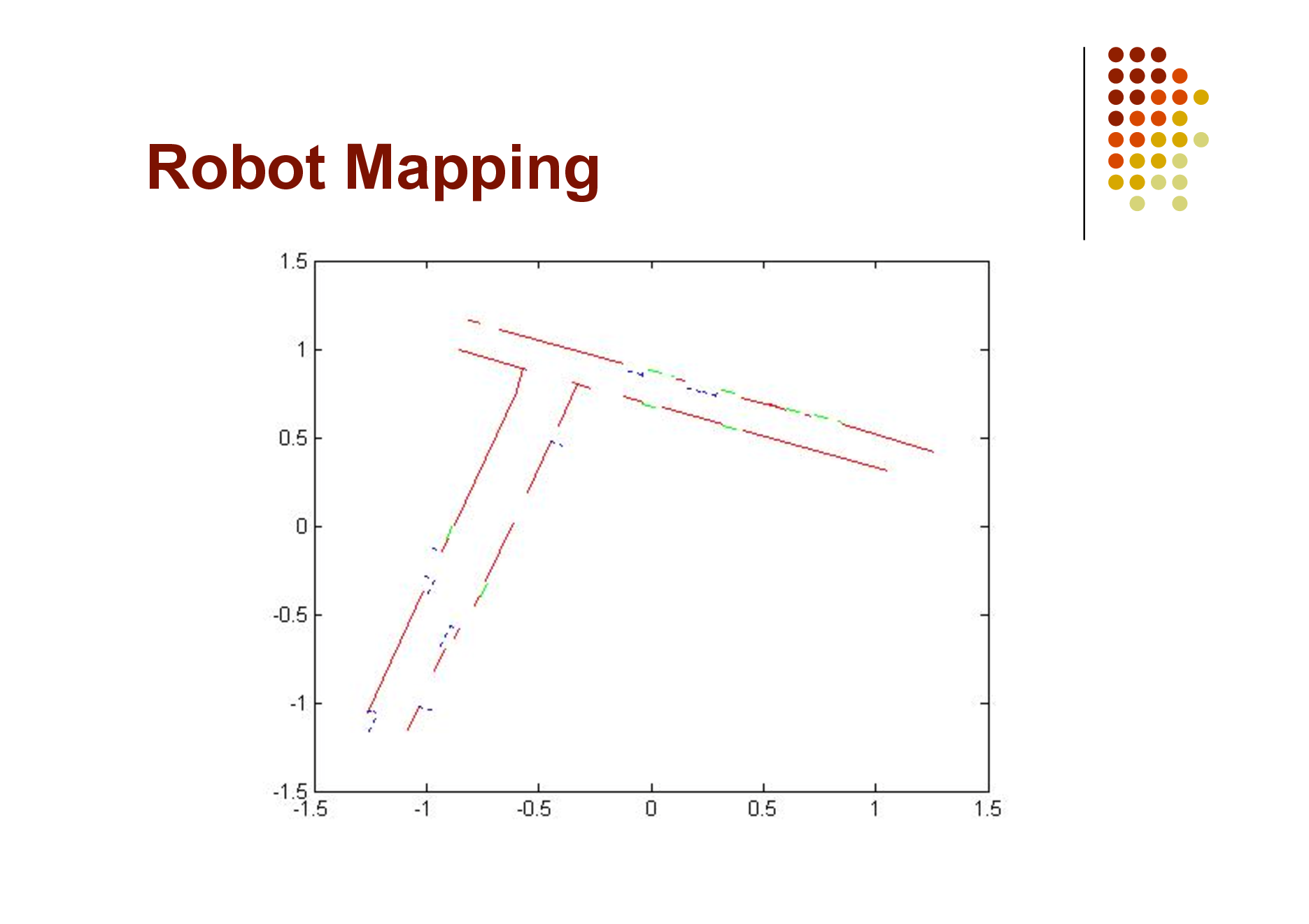
Input: Laser range finder segments (xi, yi, xf, yf) Outputs:
Segment labels (Wall, Door, Other) Assignment of wall segments to walls Position of walls (xi, yi, xf, yf)
103
Robot Mapping
104
MLNs for Hybrid Domains
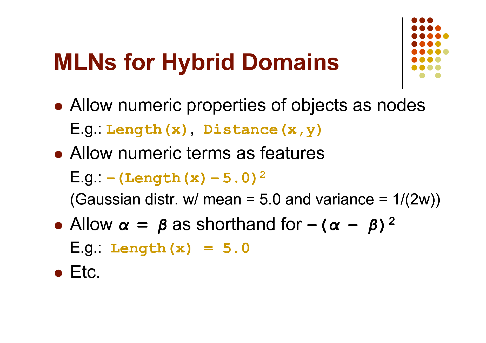
Allow numeric properties of objects as nodes
E.g.: Length(x), Distance(x,y)
Allow numeric terms as features
E.g.: (Length(x) 5.0)2 (Gaussian distr. w/ mean = 5.0 and variance = 1/(2w))
Allow = as shorthand for ( )2
E.g.: Length(x) = 5.0
Etc.
105
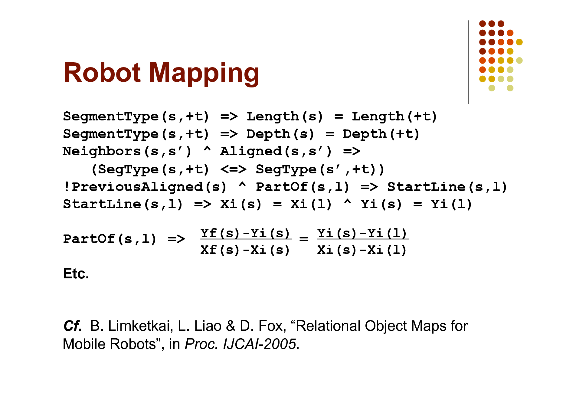
Robot Mapping
SegmentType(s,+t) => Length(s) = Length(+t) SegmentType(s,+t) => Depth(s) = Depth(+t) Neighbors(s,s) ^ Aligned(s,s) => (SegType(s,+t) <=> SegType(s,+t)) !PreviousAligned(s) ^ PartOf(s,l) => StartLine(s,l) StartLine(s,l) => Xi(s) = Xi(l) ^ Yi(s) = Yi(l) PartOf(s,l) => Etc. Cf. B. Limketkai, L. Liao & D. Fox, Relational Object Maps for Mobile Robots, in Proc. IJCAI-2005.
Yf(s)-Yi(s) = Yi(s)-Yi(l) Xf(s)-Xi(s) Xi(s)-Xi(l)
106
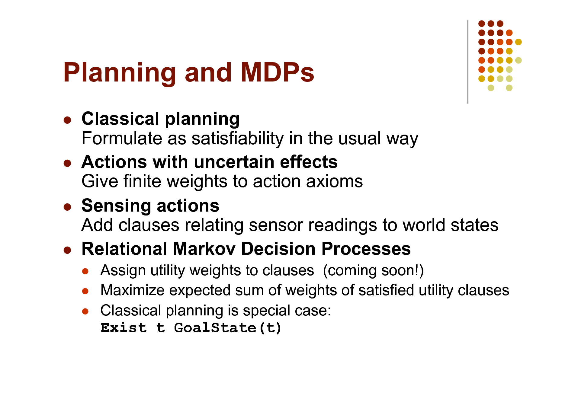
Planning and MDPs
Classical planning Formulate as satisfiability in the usual way Actions with uncertain effects Give finite weights to action axioms Sensing actions Add clauses relating sensor readings to world states Relational Markov Decision Processes
Assign utility weights to clauses (coming soon!) Maximize expected sum of weights of satisfied utility clauses Classical planning is special case: Exist t GoalState(t)
107
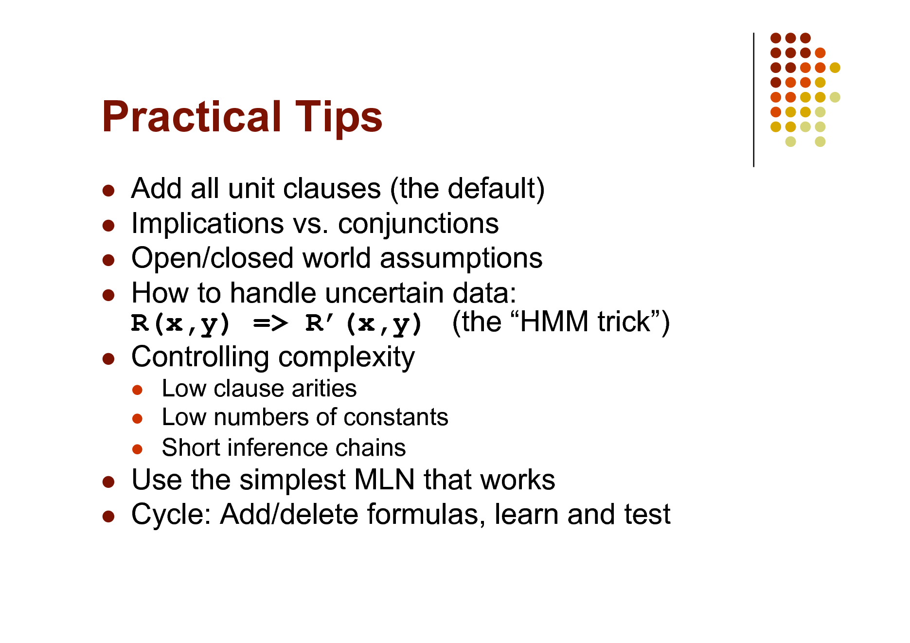
Practical Tips
Add all unit clauses (the default) Implications vs. conjunctions Open/closed world assumptions How to handle uncertain data: R(x,y) => R(x,y) (the HMM trick) Controlling complexity
Low clause arities Low numbers of constants Short inference chains
Use the simplest MLN that works Cycle: Add/delete formulas, learn and test
108
Summary
Most domains are non-i.i.d. Much progress in recent years SRL mature enough to be practical tool Many old and new research issues Check out the Alchemy Web site: alchemy.cs.washington.edu
109