Note

To run this notebook in JupyterLab, load examples/ex7_1.ipynb

Statistical Relational Learning with `pslpython`¶

In this section we'll explore one form of statistical relational learning called probabilistic soft logic (PSL).

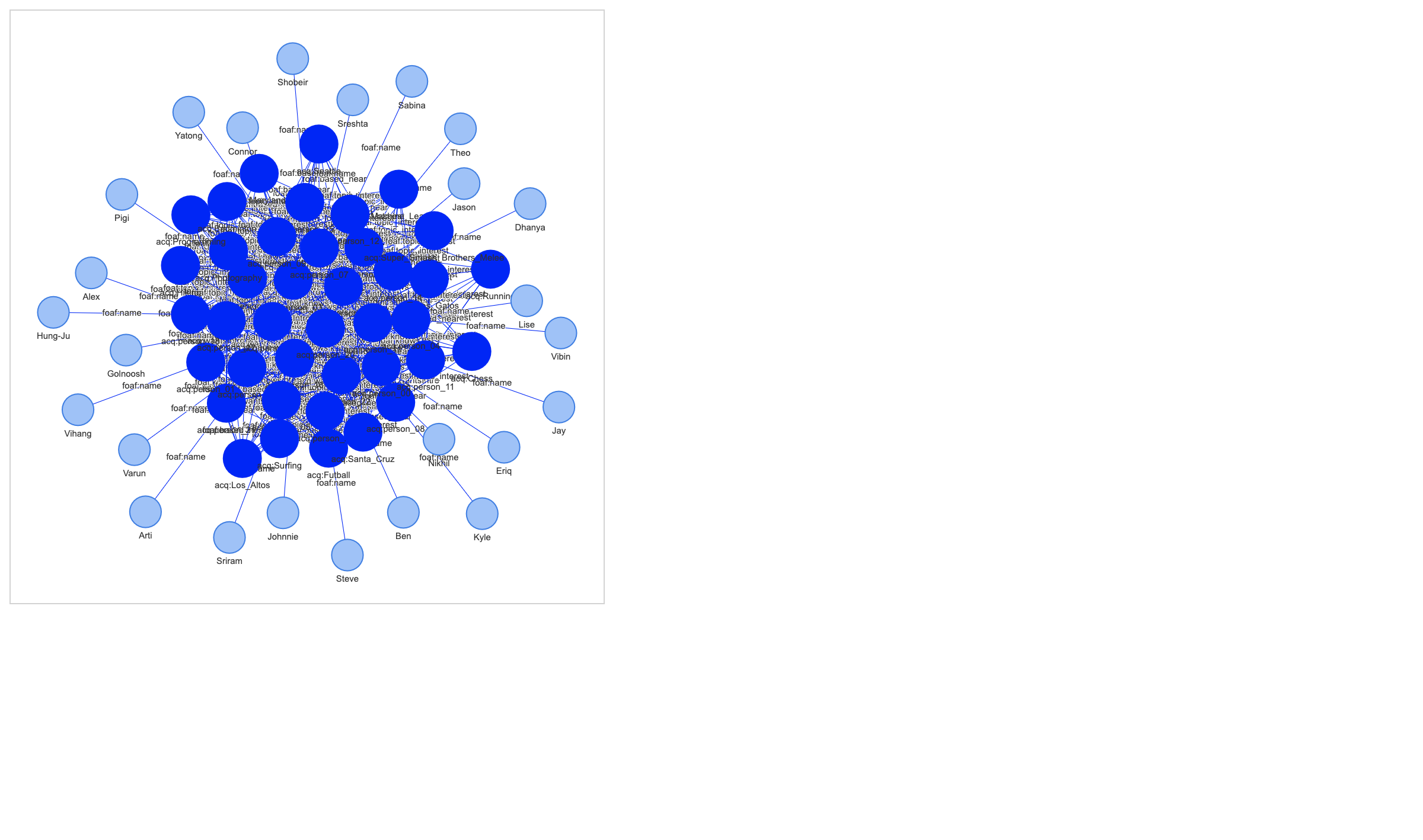
One of the examples given for PSL is called simple acquaintances, which uses a graph of some friends, where they live, what interests they share, and then infers who probably knows whom. Some people explicitly do or do not know each other, while other "knows" relations can be inferred based on whether two people have lived in the same place or share common interest.

The objective is to build a PSL model for link prediction, to evaluate the annotations in the friend graph. In this case, we'll assume that the "knows" relations have been added from a questionable source (e.g., some third-party dataset) so we'll measure a subset of these relations and determine their likelihood. NB: this is really useful for cleaning up annotations in a large graph!

Now let's load a KG which is an RDF representation of this "simple acquaintances" example, based on using the foaf vocabulary:

import kglab

namespaces = {
    "acq":  "http://example.org/stuff/",
    "foaf": "http://xmlns.com/foaf/0.1/",
    }

kg = kglab.KnowledgeGraph(
    name = "LINQS simple acquaintance example for PSL",
    base_uri = "http://example.org/stuff/",
    namespaces = namespaces,
    )

kg.load_rdf("../dat/acq.ttl")

<kglab.kglab.KnowledgeGraph at 0x10c655690>

Take a look at the dat/acq.ttl file to see the people and their relations. Here's a quick visualization of the graph:

VIS_STYLE = {
    "foaf": {
        "color": "orange",
        "size": 5,
    },
    "acq":{
        "color": "blue",
        "size": 30,
    },
}

excludes = [
    kg.get_ns("rdf").type,
    kg.get_ns("rdfs").domain,
    kg.get_ns("rdfs").range,
]

subgraph = kglab.SubgraphTensor(kg, excludes=excludes)
pyvis_graph = subgraph.build_pyvis_graph(notebook=True, style=VIS_STYLE)

pyvis_graph.force_atlas_2based()
pyvis_graph.show("tmp.fig04.html")

png

Loading a PSL model¶

Next, we'll use the pslpython library implemented in Python (atop its core library running in Java) to define three predicates (i.e., relations – similar as in RDF) which are: Neighbors, Likes, Knows

psl = kglab.PSLModel(
    name = "simple acquaintances",
    )

Then add each of the predicates:

psl.add_predicate("Lived", size=2)
psl.add_predicate("Likes", size=2)
psl.add_predicate("Knows", size=2, closed=False)

<kglab.srl.PSLModel at 0x12e7d9f10>

Next, we'll add a set of probabilistic rules, all with different weights applied:

"Two people who live in the same place are more likely to know each other"
"Two people who don't live in the same place are less likely to know each other"
"Two people who share a common interest are more likely to know each other"
"Two people who both know a third person are more likely to know each other"
"Otherwise, any pair of people are less likely to know each other"

psl.add_rule("Lived(P1, L) & Lived(P2, L) & (P1 != P2) -> Knows(P1, P2)", weight=20.0, squared=True)

psl.add_rule("Lived(P1, L1) & Lived(P2, L2) & (P1 != P2) & (L1 != L2) -> !Knows(P1, P2)", weight=5.0, squared=True)

psl.add_rule("Likes(P1, L) & Likes(P2, L) & (P1 != P2) -> Knows(P1, P2)", weight=10.0, squared=True)

psl.add_rule("Knows(P1, P2) & Knows(P2, P3) & (P1 != P3) -> Knows(P1, P3)", weight=5.0, squared=True)

psl.add_rule("!Knows(P1, P2)", weight=5.0, squared=True)

<kglab.srl.PSLModel at 0x12e7d9f10>

Finally we'll add a commutative rule such that:

"If Person 1 knows Person 2, then Person 2 also knows Person 1."

psl.add_rule("Knows(P1, P2) = Knows(P2, P1)", weighted=False)

<kglab.srl.PSLModel at 0x12e7d9f10>

To initialize the model, we'll clear any pre-existing data for each of the predicates:

psl.clear_model()

<kglab.srl.PSLModel at 0x12e7d9f10>

Next we'll create a specific Subgraph to transform the names of foaf:Person in the graph, since the PSL rules in this example focus on relations among the people:

people_iter = kg.rdf_graph().subjects(kg.get_ns("rdf").type, kg.get_ns("foaf").Person)
people_nodes = [ p for p in sorted(people_iter, key=lambda p: str(p)) ]

subgraph_people = kglab.Subgraph(kg, preload=people_nodes)

Now let's query our KG to populate data into the Liked predicate in the PSL model, based on foaf:based_near which represents people who live nearby each other:

sparql = """
SELECT DISTINCT ?p1 ?l
  WHERE {
    ?p1 foaf:based_near ?l
  }
"""

for row in kg.query(sparql):
    p1 = subgraph_people.transform(row.p1)
    l = subgraph.transform(row.l)
    psl.add_data_row("Lived", [p1, l])

Note: these data points are observations, i.e., empirical support for the probabilistic model.

Next let's query our KG to populate data into the Likes predicate in the PSL model, based on shared interests in foaf:topic_interest topics:

sparql = """
SELECT DISTINCT ?p1 ?t
  WHERE {
    ?p1 foaf:topic_interest ?t
  }
  """

for row in kg.query(sparql):
    p1 = subgraph_people.transform(row.p1)
    t = subgraph.transform(row.t)
    psl.add_data_row("Likes", [p1, t])

Just for kicks, let's take a look at the internal representation of a PSL predicate, which is a pandas.DataFrame:

predicate = psl.model.get_predicate("Likes")
predicate.__dict__

{'_types': [<ArgType.UNIQUE_STRING_ID: 'UniqueStringID'>,
  <ArgType.UNIQUE_STRING_ID: 'UniqueStringID'>],
 '_data': {<Partition.OBSERVATIONS: 'observations'>:       0   1    2
  0    13  70  1.0
  1    24  71  1.0
  2    12  72  1.0
  3     0  73  1.0
  4     7  74  1.0
  ..   ..  ..  ...
  127  10  76  1.0
  128  17  74  1.0
  129  12  71  1.0
  130   2  79  1.0
  131   5  74  1.0

  [132 rows x 3 columns],
  <Partition.TARGETS: 'targets'>: Empty DataFrame
  Columns: [0, 1, 2]
  Index: [],
  <Partition.TRUTH: 'truth'>: Empty DataFrame
  Columns: [0, 1, 2]
  Index: []},
 '_name': 'LIKES',
 '_closed': False}

df = psl.trace_predicate("Likes", partition="observations")
df

	P1	P2	value
0	0	71	1.0
1	0	72	1.0
2	0	73	1.0
3	0	74	1.0
4	0	75	1.0
...	...	...	...
127	24	74	1.0
128	24	75	1.0
129	24	76	1.0
130	24	77	1.0
131	24	78	1.0

132 rows × 3 columns

Now we'll load data from the dat/psl/knows_targets.txt CSV file, which is a list of foaf:knows relations in our graph that we want to analyze. Each of these has an assumed value of 1.0 (true) or 0.0 (false). Our PSL analysis will assign probabilities for each so that we can compare which annotations appear to be suspect and require further review:

import csv
import pandas as pd

targets = []
rows_list = []

with open("../dat/psl/knows_targets.txt", "r") as f:
    reader = csv.reader(f, delimiter="\t")

    for i, row in enumerate(reader):
        p1 = int(row[0])
        p2 = int(row[1])
        targets.append((p1, p2))

        p1_node = subgraph_people.inverse_transform(p1)
        p2_node = subgraph_people.inverse_transform(p2)

        if (p1_node, kg.get_ns("foaf").knows, p2_node) in kg.rdf_graph():
            truth = 1.0
            rows_list.append({ 0: p1, 1: p2, "truth": truth})

            psl.add_data_row("Knows", [p1, p2], partition="truth", truth_value=truth)
            psl.add_data_row("Knows", [p1, p2], partition="targets")

        elif (p1_node, kg.get_ns("acq").wantsIntro, p2_node) in kg.rdf_graph():
            truth = 0.0
            rows_list.append({ 0: p1, 1: p2, "truth": truth})

            psl.add_data_row("Knows", [p1, p2], partition="truth", truth_value=truth)
            psl.add_data_row("Knows", [p1, p2], partition="targets")

        else:
            print("UNKNOWN", p1, p2)

Here are data points which are considered ground atoms, each with a truth value set initially.

Here are also our targets for which nodes in the graph to analyze based on the rules. We'll keep a dataframe called df_dat to preserve these values for later use:

df_dat = pd.DataFrame(rows_list)
df_dat.head()

	1	truth
0	1	1.0
1	7	1.0
2	15	1.0
3	18	1.0
4	22	0.0

Next, we'll add foaf:knows observations which are in the graph, although not among our set of targets. This provides more evidence for the probabilistic inference. Note that since RDF does not allow for representing probabilities on relations, we're using the acq:wantsIntro to represent a foaf:knows with a 0.0 probability:

sparql = """
SELECT ?p1 ?p2
  WHERE {
    ?p1 foaf:knows ?p2 .
  }
  ORDER BY ?p1 ?p2
  """

for row in kg.query(sparql):
    p1 = subgraph_people.transform(row.p1)
    p2 = subgraph_people.transform(row.p2)

    if (p1, p2) not in targets:
        psl.add_data_row("Knows", [p1, p2], truth_value=1.0)

sparql = """
SELECT ?p1 ?p2
  WHERE {
    ?p1 acq:wantsIntro ?p2 .
  }
  ORDER BY ?p1 ?p2
  """

for row in kg.query(sparql):
    p1 = subgraph_people.transform(row.p1)
    p2 = subgraph_people.transform(row.p2)

    if (p1, p2) not in targets:
        psl.add_data_row("Knows", [p1, p2], truth_value=0.0)

Now we're ready to run optimization on the PSL model and infer the grounded atoms. This may take a few minutes to run:

psl.infer()

7610 [pslpython.model PSL] INFO --- 0    [main] INFO  org.linqs.psl.cli.Launcher  - Running PSL CLI Version 2.2.2-5f9a472
7915 [pslpython.model PSL] INFO --- 308  [main] INFO  org.linqs.psl.cli.Launcher  - Loading data
8134 [pslpython.model PSL] INFO --- 527  [main] INFO  org.linqs.psl.cli.Launcher  - Data loading complete
8135 [pslpython.model PSL] INFO --- 527  [main] INFO  org.linqs.psl.cli.Launcher  - Loading model from /var/folders/zz/2ffrqd5j7n52x67qd94h_r_h0000gp/T/psl-python/simple acquaintances/simple acquaintances.psl
8279 [pslpython.model PSL] INFO --- 672  [main] INFO  org.linqs.psl.cli.Launcher  - Model loading complete
8281 [pslpython.model PSL] INFO --- 673  [main] INFO  org.linqs.psl.cli.Launcher  - Starting inference with class: org.linqs.psl.application.inference.MPEInference
8456 [pslpython.model PSL] INFO --- 849  [main] INFO  org.linqs.psl.application.inference.MPEInference  - Grounding out model.
8836 [pslpython.model PSL] INFO --- 1229 [main] INFO  org.linqs.psl.application.inference.MPEInference  - Grounding complete.
8895 [pslpython.model PSL] INFO --- 1288 [main] INFO  org.linqs.psl.application.inference.InferenceApplication  - Beginning inference.
9544 [pslpython.model PSL] WARNING --- 1937 [main] WARN  org.linqs.psl.reasoner.admm.ADMMReasoner  - No feasible solution found. 34 constraints violated.
9545 [pslpython.model PSL] INFO --- 1937 [main] INFO  org.linqs.psl.reasoner.admm.ADMMReasoner  - Optimization completed in 1009 iterations. Objective: 7542.3438, Feasible: false, Primal res.: 0.053799044, Dual res.: 0.0010063195
9546 [pslpython.model PSL] INFO --- 1937 [main] INFO  org.linqs.psl.application.inference.InferenceApplication  - Inference complete.
9547 [pslpython.model PSL] INFO --- 1938 [main] INFO  org.linqs.psl.application.inference.InferenceApplication  - Writing results to Database.
9594 [pslpython.model PSL] INFO --- 1987 [main] INFO  org.linqs.psl.application.inference.InferenceApplication  - Results committed to database.
9595 [pslpython.model PSL] INFO --- 1987 [main] INFO  org.linqs.psl.cli.Launcher  - Inference Complete

Let's examine the results. We'll get a pandas.DataFrame describing the targets in the Knows predicate:

df = psl.get_results("Knows")
df.head()

	predicate	0	1	truth
0	KNOWS	7	20	0.002160
1	KNOWS	8	13	0.997971
2	KNOWS	8	12	0.995324
3	KNOWS	8	10	0.996841
4	KNOWS	8	21	0.997979

Now we can compare the "truth" values from our targets, with their probabilities from the inference provided by the PSL model. Let's build a dataframe to show that:

dat_val = {}
df.insert(1, "p1", "")
df.insert(2, "p2", "")

for index, row in df_dat.iterrows():
    p1 = int(row[0])
    p2 = int(row[1])
    key = (p1, p2)
    dat_val[key] = row["truth"]

for index, row in df.iterrows():
    p1 = int(row[0])
    p2 = int(row[1])
    key = (p1, p2)

    df.at[index, "diff"] = row["truth"] - dat_val[key]
    df.at[index, "p1"] = str(subgraph_people.inverse_transform(p1))
    df.at[index, "p2"] = str(subgraph_people.inverse_transform(p2))

df = df.drop(df.columns[[3, 4]], axis=1)
pd.set_option("max_rows", None)

df.head()

	predicate	p1	p2	truth	diff
0	KNOWS	http://example.org/stuff/person_07	http://example.org/stuff/person_20	0.002160	0.002160
1	KNOWS	http://example.org/stuff/person_08	http://example.org/stuff/person_13	0.997971	-0.002029
2	KNOWS	http://example.org/stuff/person_08	http://example.org/stuff/person_12	0.995324	-0.004676
3	KNOWS	http://example.org/stuff/person_08	http://example.org/stuff/person_10	0.996841	-0.003159
4	KNOWS	http://example.org/stuff/person_08	http://example.org/stuff/person_21	0.997979	-0.002021

In other words, which of these "knows" relations in the graph appears to be suspect, based on our rules plus the other evidence in the graph?

Let's visualize a histogram of how the inferred probabilities are distributed:

df["diff"].hist();

png

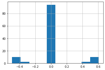
In most cases there is little or no difference in the probabilities for the target relations. However, some appear to be off by a substantial (0.6) amount, which indicates potential problems in this part of our graph data.

The following rows show where these foaf:knows annotations in the graph differs significantly from their truth values predicted by PSL:

df[df["diff"] >= 0.4]

	predicate	p1	p2	truth	diff
5	KNOWS	http://example.org/stuff/person_09	http://example.org/stuff/person_19	0.540309	0.540309
11	KNOWS	http://example.org/stuff/person_01	http://example.org/stuff/person_17	0.578482	0.578482
13	KNOWS	http://example.org/stuff/person_21	http://example.org/stuff/person_17	0.476275	0.476275
33	KNOWS	http://example.org/stuff/person_06	http://example.org/stuff/person_14	0.506647	0.506647
43	KNOWS	http://example.org/stuff/person_14	http://example.org/stuff/person_06	0.507944	0.507944
53	KNOWS	http://example.org/stuff/person_17	http://example.org/stuff/person_01	0.581062	0.581062
57	KNOWS	http://example.org/stuff/person_19	http://example.org/stuff/person_09	0.539307	0.539307
75	KNOWS	http://example.org/stuff/person_17	http://example.org/stuff/person_18	0.561153	0.561153
76	KNOWS	http://example.org/stuff/person_17	http://example.org/stuff/person_21	0.476655	0.476655
79	KNOWS	http://example.org/stuff/person_18	http://example.org/stuff/person_17	0.560538	0.560538
87	KNOWS	http://example.org/stuff/person_09	http://example.org/stuff/person_06	0.607745	0.607745
116	KNOWS	http://example.org/stuff/person_06	http://example.org/stuff/person_09	0.606495	0.606495

In most of these cases, the truth value is floating (somewhere near ~0.5) when it was expected to be zero (i.e., they don't know each other). Part of that likely comes from the use of the Likes predicate with boolean values; the original demo had probabilities for those, but was simplified here.

Speaking of human-in-the-loop practices for AI, using PSL along with a KG seems like a great way to leverage machine learning, so that the people can focus on parts of the graph that have the most uncertainty. And, therefore, probably provide the best ROI for investing time+cost into curation.

Exercises¶

Exercise 1:

Build a PSL model that tests the "noodle vs. pancake" rules used in an earlier example with our recipe KG. Which recipes should be annotated differently?

Exercise 2:

Try representing one of the other PSL examples using RDF and kglab.

Last update: 2021-04-10

	P1	P2	value
0	0	71	1.0
1	0	72	1.0
2	0	73	1.0
3	0	74	1.0
4	0	75	1.0
...	...	...	...
127	24	74	1.0
128	24	75	1.0
129	24	76	1.0
130	24	77	1.0
131	24	78	1.0

	P1	P2	value
0	0	71	1.0
1	0	72	1.0
2	0	73	1.0
3	0	74	1.0
4	0	75	1.0
...	...	...	...
127	24	74	1.0
128	24	75	1.0
129	24	76	1.0
130	24	77	1.0
131	24	78	1.0

Statistical Relational Learning with pslpython¶

Loading a PSL model¶

Exercises¶

Statistical Relational Learning with `pslpython`¶

	P1	P2	value
0	0	71	1.0
1	0	72	1.0
2	0	73	1.0
3	0	74	1.0
4	0	75	1.0
...	...	...	...
127	24	74	1.0
128	24	75	1.0
129	24	76	1.0
130	24	77	1.0
131	24	78	1.0